Sequence of event tables

This combines a sequence of event tables.

etSeq(..., samples = c("clear", "use"), waitII = c("smart", "+ii"), ii = 24)

# S3 method for rxEt
seq(...)

Arguments

...	The event tables and optionally time between event tables, called waiting times in this help document.
samples	How to handle samples when repeating an event table. The options are: "clear" Clear sampling records before combining the datasets "use" Use the sampling records when combining the datasets
waitII	This determines how waiting times between events are handled. The options are: "smart" This "smart" handling of waiting times is the default option. In this case, if the waiting time is above the last observed inter-dose interval in the first combined event table, then the actual time between doses is given by the wait time. If it is smaller than the last observed inter-dose interval, the time between event tables is given by the inter-dose interval + the waiting time between event tables. "+ii" In this case, the wait time is added to the inter-dose interval no matter the length of the wait time or inter-dose interval
ii	If there was no inter-dose intervals found in the event table, assume that the interdose interval is given by this ii value. By default this is 24.

Value

An event table

Details

This sequences all the event tables in added in the argument list .... By default when combining the event tables the offset is at least by the last inter-dose interval in the prior event table (or ii). If you separate any of the event tables by a number, the event tables will be separated at least the wait time defined by that number or the last inter-dose interval.

References

Wang W, Hallow K, James D (2015). "A Tutorial on RxODE: Simulating Differential Equation Pharmacometric Models in R." CPT: Pharmacometrics \& Systems Pharmacology, 5(1), 3-10. ISSN 2163-8306, <URL: https://www.ncbi.nlm.nih.gov/pmc/articles/PMC4728294/>.

See also

eventTable, add.sampling, add.dosing, et, etRep, etRbind, RxODE

Author

Matthew L Fidler, Wenping Wang

Examples

# \donttest{

library(RxODE)
library(units)

## Model from RxODE tutorial
mod1 <-RxODE({
    KA=2.94E-01;
    CL=1.86E+01;
    V2=4.02E+01;
    Q=1.05E+01;
    V3=2.97E+02;
    Kin=1;
    Kout=1;
    EC50=200;
    C2 = centr/V2;
    C3 = peri/V3;
    d/dt(depot) =-KA*depot;
    d/dt(centr) = KA*depot - CL*C2 - Q*C2 + Q*C3;
    d/dt(peri)  =                    Q*C2 - Q*C3;
    d/dt(eff)  = Kin - Kout*(1-C2/(EC50+C2))*eff;
});
#>  

## These are making the more complex regimens of the RxODE tutorial

## bid for 5 days
bid <- et(timeUnits="hr") %>%
       et(amt=10000,ii=12,until=set_units(5, "days"))

## qd for 5 days
qd <- et(timeUnits="hr") %>%
      et(amt=20000,ii=24,until=set_units(5, "days"))

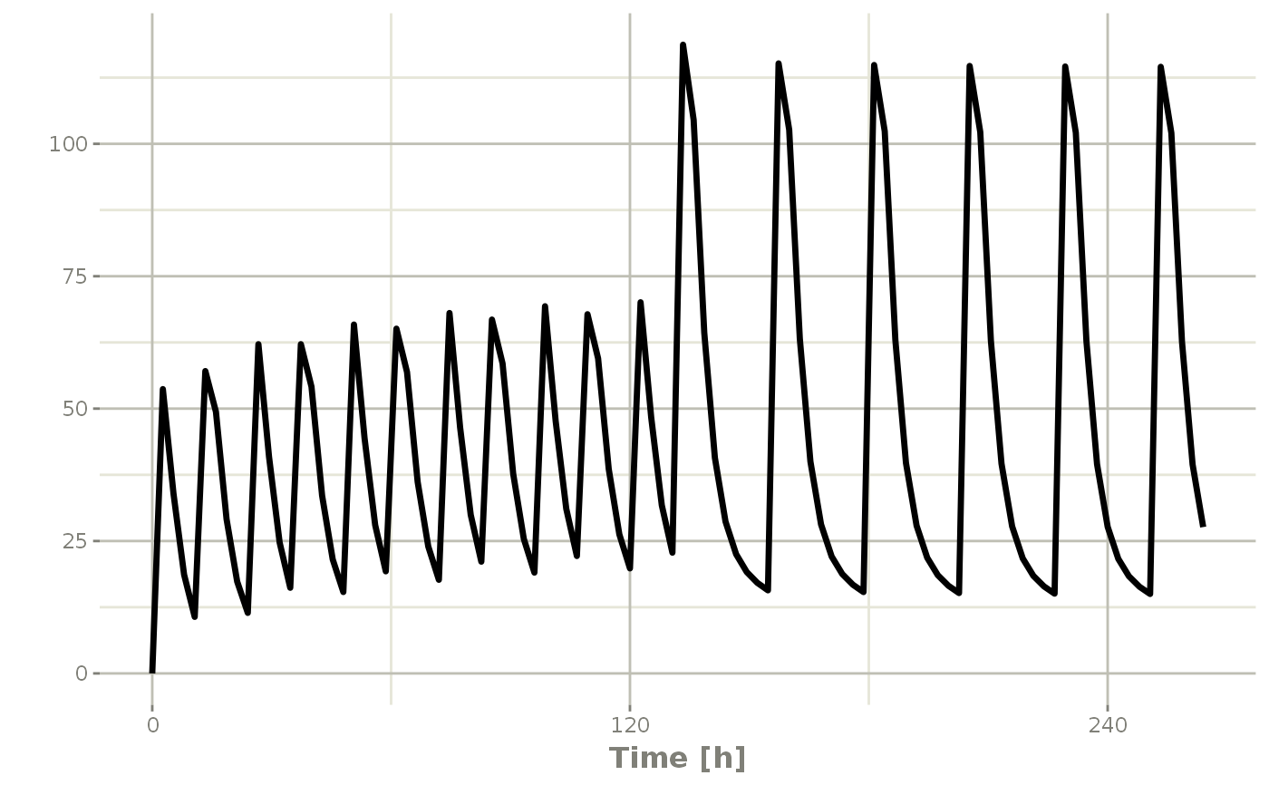
## bid for 5 days followed by qd for 5 days

et <- seq(bid,qd) %>% et(seq(0,11*24,length.out=100));

bidQd <- rxSolve(mod1, et)

plot(bidQd, C2)



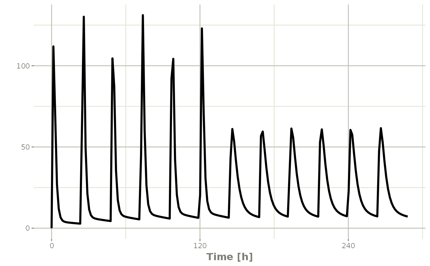
## Now Infusion for 5 days followed by oral for 5 days

##  note you can dose to a named compartment instead of using the compartment number
infusion <- et(timeUnits = "hr") %>%
      et(amt=10000, rate=5000, ii=24, until=set_units(5, "days"), cmt="centr")


qd <- et(timeUnits = "hr") %>% et(amt=10000, ii=24, until=set_units(5, "days"), cmt="depot")

et <- seq(infusion,qd)

infusionQd <- rxSolve(mod1, et)

plot(infusionQd, C2)


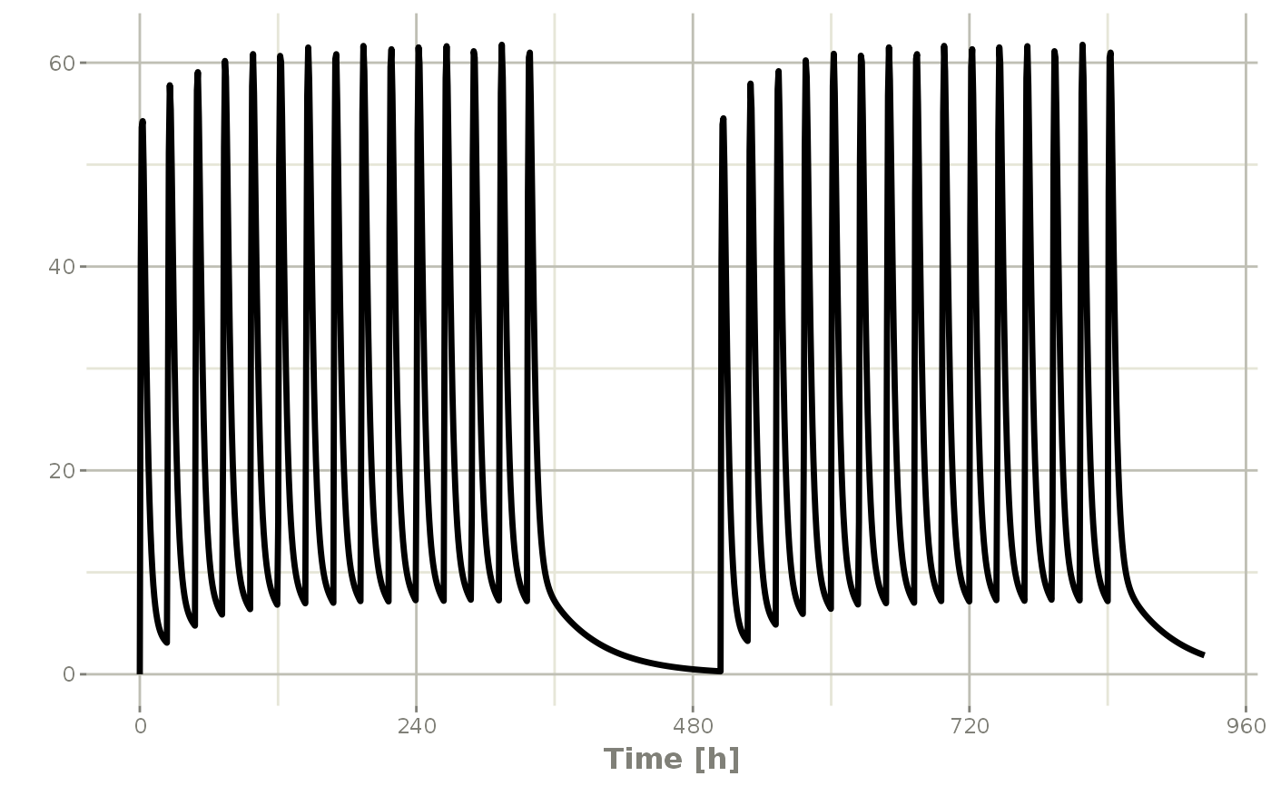
## 2wk-on, 1wk-off

qd <- et(timeUnits = "hr") %>% et(amt=10000, ii=24, until=set_units(2, "weeks"), cmt="depot")

et <- seq(qd, set_units(1,"weeks"), qd) %>%
     add.sampling(set_units(seq(0, 5.5,by=0.005),weeks))

wkOnOff <- rxSolve(mod1, et)

plot(wkOnOff, C2)


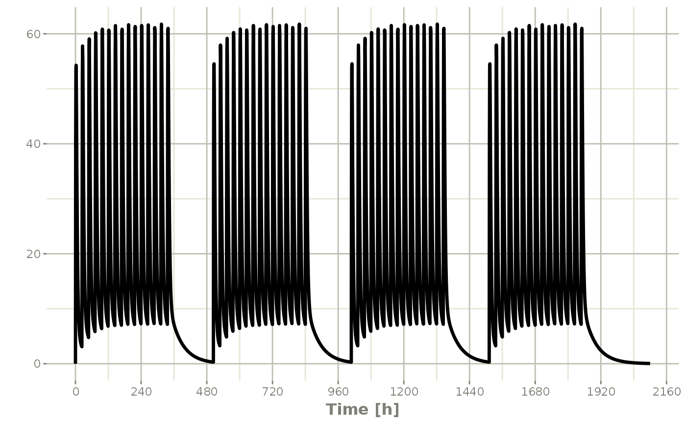
## You can also repeat the cycle easily with the rep function

qd <-et(timeUnits = "hr") %>% et(amt=10000, ii=24, until=set_units(2, "weeks"), cmt="depot")

et <- etRep(qd, times=4, wait=set_units(1,"weeks")) %>%
     add.sampling(set_units(seq(0, 12.5,by=0.005),weeks))

repCycle4 <- rxSolve(mod1, et)

plot(repCycle4, C2)


# }