Individual Covariates

If there is an individual covariate you wish to solve for you may specify it by the iCov dataset:

library(RxODE)

## RxODE 1.1.1 using 1 threads (see ?getRxThreads)
##   no cache: create with `rxCreateCache()`

library(units)

## udunits database from /usr/share/xml/udunits/udunits2.xml

library(xgxr)

mod3 <- RxODE({
    KA=2.94E-01;
    ## Clearance with individuals
    CL=1.86E+01 * (WT / 70) ^ 0.75;
    V2=4.02E+01;
    Q=1.05E+01;
    V3=2.97E+02;
    Kin=1;
    Kout=1;
    EC50=200;
    ## The linCmt() picks up the variables from above
    C2   = linCmt();
    Tz= 8
    amp=0.1
    eff(0) = 1  ## This specifies that the effect compartment starts at 1.
    d/dt(eff) =  Kin - Kout*(1-C2/(EC50+C2))*eff;
})

ev <- et(amount.units="mg", time.units="hours") %>%
    et(amt=10000, cmt=1) %>%
    et(0,48,length.out=100) %>%
    et(id=1:4);

set.seed(10)
rxSetSeed(10)
## Now use iCov to simulate a 4-id sample
r1 <- solve(mod3, ev,
            # Create individual covariate data-frame
            iCov=data.frame(id=1:4, WT=rnorm(4, 70, 10)),
            # in this case it would be useful to keep the WT in the output dataset
            keep="WT")
print(r1)

## ▂▂▂▂▂▂▂▂▂▂▂▂▂▂▂▂▂▂▂▂▂▂▂▂▂▂▂▂▂▂ Solved RxODE object ▂▂▂▂▂▂▂▂▂▂▂▂▂▂▂▂▂▂▂▂▂▂▂▂▂▂▂▂▂
## ── Parameters ($params): ───────────────────────────────────────────────────────
##      KA      V2       Q      V3     Kin    Kout    EC50      Tz     amp 
##   0.294  40.200  10.500 297.000   1.000   1.000 200.000   8.000   0.100 
## ── Initial Conditions ($inits): ────────────────────────────────────────────────
## eff 
##   1 
## ── First part of data (object): ────────────────────────────────────────────────
## # A tibble: 400 × 6
##      id  time    CL    C2   eff    WT
##   <int>   [h] <dbl> <dbl> <dbl> <dbl>
## 1     1 0      18.6   0    1     70.2
## 2     1 0.485  18.6  27.8  1.03  70.2
## 3     1 0.970  18.6  43.7  1.08  70.2
## 4     1 1.45   18.6  51.7  1.13  70.2
## 5     1 1.94   18.6  54.7  1.18  70.2
## 6     1 2.42   18.6  54.5  1.21  70.2
## # … with 394 more rows
## ▂▂▂▂▂▂▂▂▂▂▂▂▂▂▂▂▂▂▂▂▂▂▂▂▂▂▂▂▂▂▂▂▂▂▂▂▂▂▂▂▂▂▂▂▂▂▂▂▂▂▂▂▂▂▂▂▂▂▂▂▂▂▂▂▂▂▂▂▂▂▂▂▂▂▂▂▂▂▂▂

plot(r1, C2, log="y")

## Warning: Transformation introduced infinite values in continuous y-axis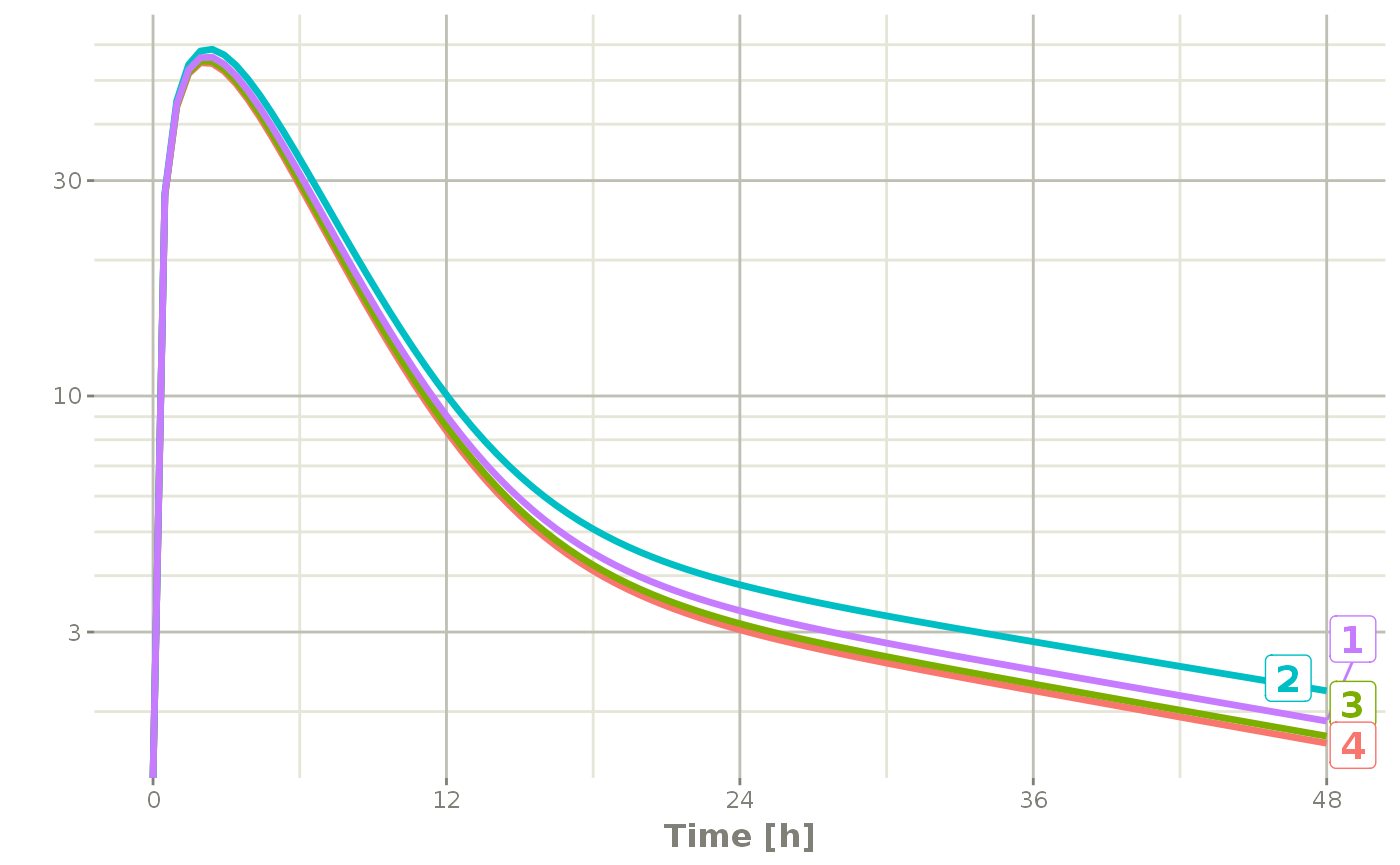

Time Varying Covariates

Covariates are easy to specify in RxODE, you can specify them as a variable. Time-varying covariates, like clock time in a circadian rhythm model, can also be used. Extending the indirect response model already discussed, we have:

library(RxODE)
library(units)

mod3 <- RxODE({
    KA=2.94E-01;
    CL=1.86E+01;
    V2=4.02E+01;
    Q=1.05E+01;
    V3=2.97E+02;
    Kin0=1;
    Kout=1;
    EC50=200;
    ## The linCmt() picks up the variables from above
    C2   = linCmt();
    Tz= 8
    amp=0.1
    eff(0) = 1  ## This specifies that the effect compartment starts at 1.
    ## Kin changes based on time of day (like cortosol)
    Kin =   Kin0 +amp *cos(2*pi*(ctime-Tz)/24)
    d/dt(eff) =  Kin - Kout*(1-C2/(EC50+C2))*eff;
})


ev <- eventTable(amount.units="mg", time.units="hours") %>%
    add.dosing(dose=10000, nbr.doses=1, dosing.to=1) %>%
    add.sampling(seq(0,48,length.out=100));


## Create data frame of 8 am dosing for the first dose This is done
## with base R but it can be done with dplyr or data.table
ev$ctime <- (ev$time+set_units(8,hr)) %% 24

Now there is a covariate present in the event dataset, the system can be solved by combining the dataset and the model:

r1 <- solve(mod3, ev, covs_interpolation="linear")
print(r1)
#> ▂▂▂▂▂▂▂▂▂▂▂▂▂▂▂▂▂▂▂▂▂▂▂▂▂▂▂▂▂▂ Solved RxODE object ▂▂▂▂▂▂▂▂▂▂▂▂▂▂▂▂▂▂▂▂▂▂▂▂▂▂▂▂▂
#> ── Parameters ($params): ───────────────────────────────────────────────────────
#>         KA         CL         V2          Q         V3       Kin0       Kout 
#>   0.294000  18.600000  40.200000  10.500000 297.000000   1.000000   1.000000 
#>       EC50         Tz        amp         pi 
#> 200.000000   8.000000   0.100000   3.141593 
#> ── Initial Conditions ($inits): ────────────────────────────────────────────────
#> eff 
#>   1 
#> ── First part of data (object): ────────────────────────────────────────────────
#> # A tibble: 100 × 4
#>    time    C2   Kin   eff
#>     [h] <dbl> <dbl> <dbl>
#> 1 0       0    1.1   1   
#> 2 0.485  27.8  1.10  1.07
#> 3 0.970  43.7  1.10  1.15
#> 4 1.45   51.8  1.09  1.22
#> 5 1.94   54.8  1.09  1.27
#> 6 2.42   54.6  1.08  1.30
#> # … with 94 more rows
#> ▂▂▂▂▂▂▂▂▂▂▂▂▂▂▂▂▂▂▂▂▂▂▂▂▂▂▂▂▂▂▂▂▂▂▂▂▂▂▂▂▂▂▂▂▂▂▂▂▂▂▂▂▂▂▂▂▂▂▂▂▂▂▂▂▂▂▂▂▂▂▂▂▂▂▂▂▂▂▂▂

When solving ODE equations, the solver may sample times outside of the data. When this happens, this ODE solver can use linear interpolation between the covariate values. It is equivalent to R’s approxfun with method="linear".

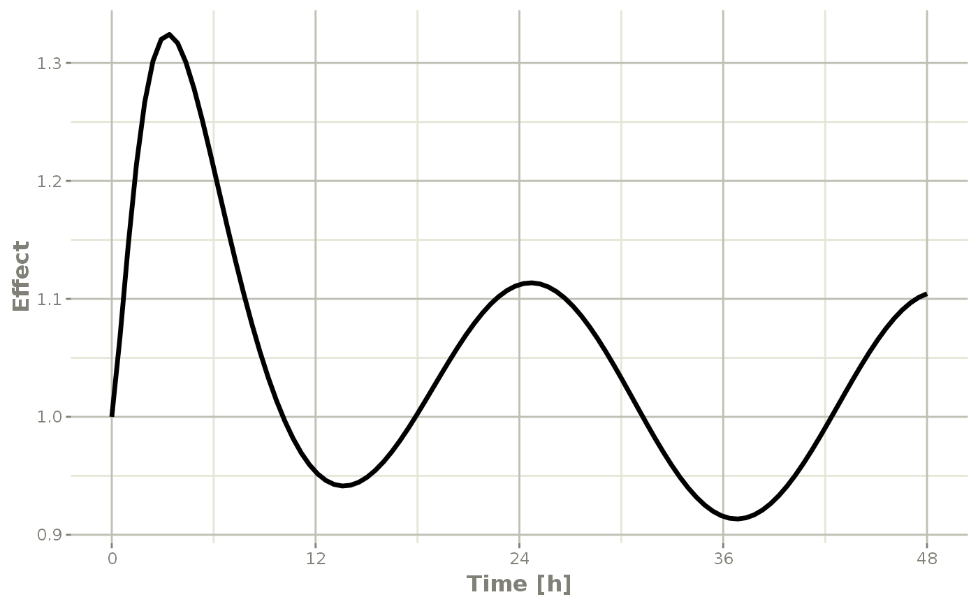
plot(r1,C2, ylab="Central Concentration")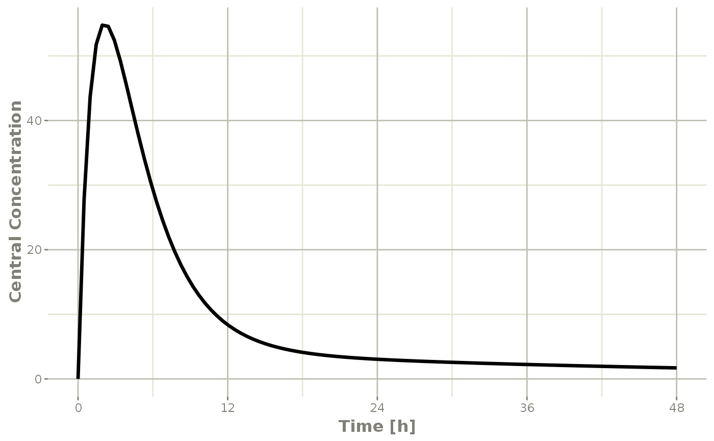

plot(r1,eff) + ylab("Effect") + xlab("Time");

Note that the linear approximation in this case leads to some kinks in the solved system at 24-hours where the covariate has a linear interpolation between near 24 and near 0. While linear seems reasonable, cases like clock time make other interpolation methods more attractive.

In RxODE the default covariate interpolation is be the last observation carried forward (locf), or constant approximation. This is equivalent to R’s approxfun with method="constant".

r1 <- solve(mod3, ev,covs_interpolation="constant")
print(r1)
#> ▂▂▂▂▂▂▂▂▂▂▂▂▂▂▂▂▂▂▂▂▂▂▂▂▂▂▂▂▂▂ Solved RxODE object ▂▂▂▂▂▂▂▂▂▂▂▂▂▂▂▂▂▂▂▂▂▂▂▂▂▂▂▂▂
#> ── Parameters ($params): ───────────────────────────────────────────────────────
#>         KA         CL         V2          Q         V3       Kin0       Kout 
#>   0.294000  18.600000  40.200000  10.500000 297.000000   1.000000   1.000000 
#>       EC50         Tz        amp         pi 
#> 200.000000   8.000000   0.100000   3.141593 
#> ── Initial Conditions ($inits): ────────────────────────────────────────────────
#> eff 
#>   1 
#> ── First part of data (object): ────────────────────────────────────────────────
#> # A tibble: 100 × 4
#>    time    C2   Kin   eff
#>     [h] <dbl> <dbl> <dbl>
#> 1 0       0    1.1   1   
#> 2 0.485  27.8  1.10  1.07
#> 3 0.970  43.7  1.10  1.15
#> 4 1.45   51.8  1.09  1.22
#> 5 1.94   54.8  1.09  1.27
#> 6 2.42   54.6  1.08  1.31
#> # … with 94 more rows
#> ▂▂▂▂▂▂▂▂▂▂▂▂▂▂▂▂▂▂▂▂▂▂▂▂▂▂▂▂▂▂▂▂▂▂▂▂▂▂▂▂▂▂▂▂▂▂▂▂▂▂▂▂▂▂▂▂▂▂▂▂▂▂▂▂▂▂▂▂▂▂▂▂▂▂▂▂▂▂▂▂

which gives the following plots:

plot(r1,C2, ylab="Central Concentration", xlab="Time")

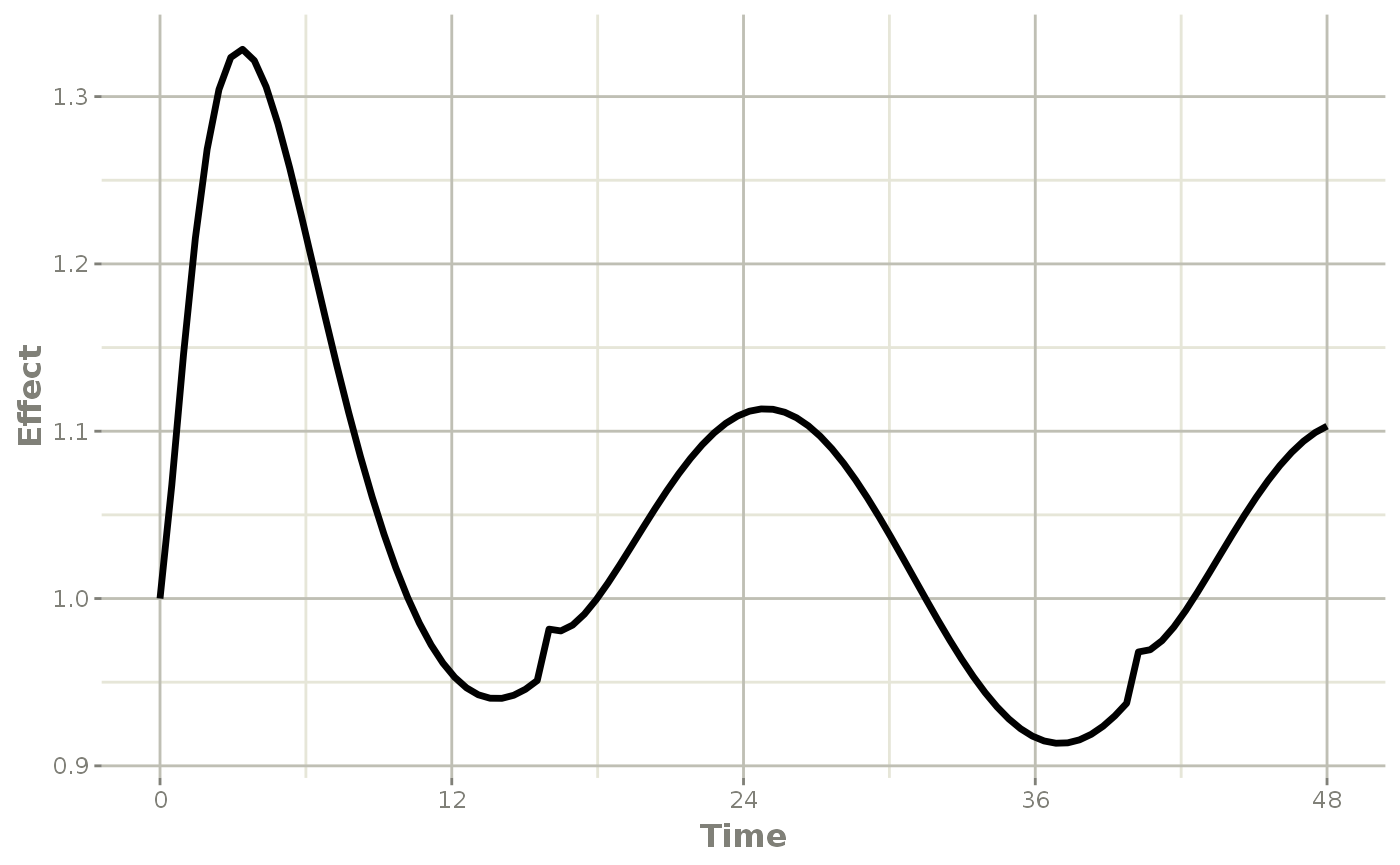
plot(r1,eff, ylab="Effect", xlab="Time")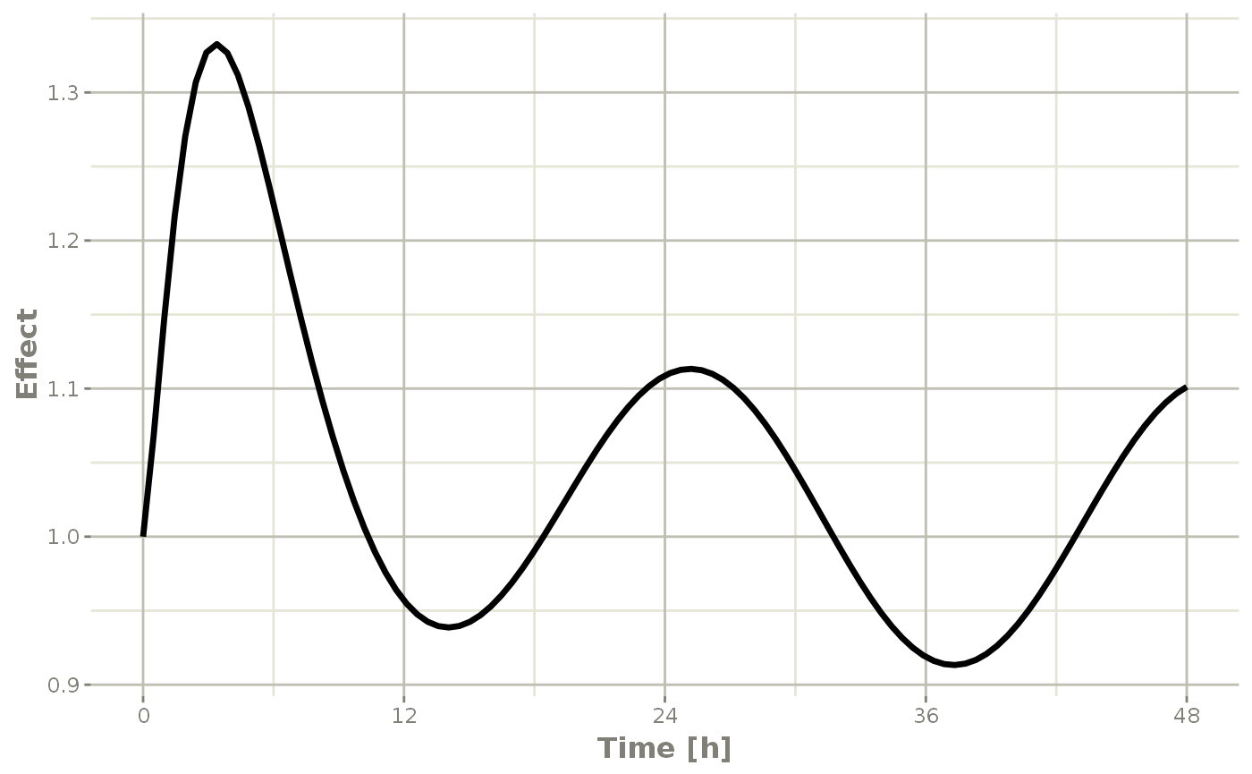

In this case, the plots seem to be smoother.

You can also use NONMEM’s preferred interpolation style of next observation carried backward (NOCB):

r1 <- solve(mod3, ev,covs_interpolation="nocb")
print(r1)
#> ▂▂▂▂▂▂▂▂▂▂▂▂▂▂▂▂▂▂▂▂▂▂▂▂▂▂▂▂▂▂ Solved RxODE object ▂▂▂▂▂▂▂▂▂▂▂▂▂▂▂▂▂▂▂▂▂▂▂▂▂▂▂▂▂
#> ── Parameters ($params): ───────────────────────────────────────────────────────
#>         KA         CL         V2          Q         V3       Kin0       Kout 
#>   0.294000  18.600000  40.200000  10.500000 297.000000   1.000000   1.000000 
#>       EC50         Tz        amp         pi 
#> 200.000000   8.000000   0.100000   3.141593 
#> ── Initial Conditions ($inits): ────────────────────────────────────────────────
#> eff 
#>   1 
#> ── First part of data (object): ────────────────────────────────────────────────
#> # A tibble: 100 × 4
#>    time    C2   Kin   eff
#>     [h] <dbl> <dbl> <dbl>
#> 1 0       0    1.1   1   
#> 2 0.485  27.8  1.10  1.07
#> 3 0.970  43.7  1.10  1.15
#> 4 1.45   51.8  1.09  1.21
#> 5 1.94   54.8  1.09  1.27
#> 6 2.42   54.6  1.08  1.30
#> # … with 94 more rows
#> ▂▂▂▂▂▂▂▂▂▂▂▂▂▂▂▂▂▂▂▂▂▂▂▂▂▂▂▂▂▂▂▂▂▂▂▂▂▂▂▂▂▂▂▂▂▂▂▂▂▂▂▂▂▂▂▂▂▂▂▂▂▂▂▂▂▂▂▂▂▂▂▂▂▂▂▂▂▂▂▂

which gives the following plots:

plot(r1,C2, ylab="Central Concentration", xlab="Time")

plot(r1,eff, ylab="Effect", xlab="Time")

RxODE Covariates

2021-09-01

Individual Covariates

Time Varying Covariates