RxODE Transit Compartment Models

2021-09-01

Savic 2008 first introduced the idea of transit compartments being a mechanistic explanation of a a lag-time type phenomena. RxODE has special handling of these models:

You can specify this in a similar manner as the original paper:

library(RxODE)

## RxODE 1.1.1 using 1 threads (see ?getRxThreads)
##   no cache: create with `rxCreateCache()`

mod <- RxODE({
    ## Table 3 from Savic 2007
    cl = 17.2 # (L/hr)
    vc = 45.1 # L
    ka = 0.38 # 1/hr
    mtt = 0.37 # hr
    bio=1
    n = 20.1
    k = cl/vc
    ktr = (n+1)/mtt
    ## note that lgammafn is the same as lgamma in R.
    d/dt(depot) = exp(log(bio*podo)+log(ktr)+n*log(ktr*t)-ktr*t-lgammafn(n+1))-ka*depot
    d/dt(cen) = ka*depot-k*cen
})

et <- eventTable();
et$add.sampling(seq(0, 7, length.out=200));
et$add.dosing(20, start.time=0);

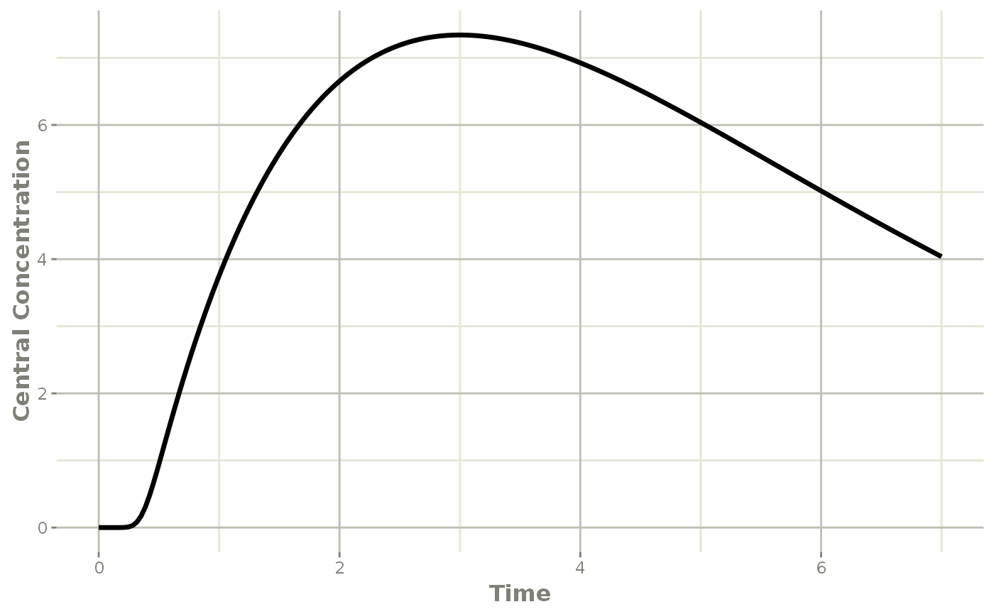
transit <- rxSolve(mod, et, transit_abs=TRUE)

plot(transit, cen, ylab="Central Concentration")

Another option is to specify the transit compartment function transit syntax. This specifies the parameters transit(number of transit compartments, mean transit time, bioavailability). The bioavailability term is optional.

Using the transit code also automatically turns on the transit_abs option. Therefore, the same model can be specified by:

mod <- RxODE({
    ## Table 3 from Savic 2007
    cl = 17.2 # (L/hr)
    vc = 45.1 # L
    ka = 0.38 # 1/hr
    mtt = 0.37 # hr
    bio=1
    n = 20.1
    k = cl/vc
    ktr = (n+1)/mtt
    d/dt(depot) = transit(n,mtt,bio)-ka*depot
    d/dt(cen) = ka*depot-k*cen
})

et <- eventTable();
et$add.sampling(seq(0, 7, length.out=200));
et$add.dosing(20, start.time=0);

transit <- rxSolve(mod, et)

## Warning: assumed transit compartment model since 'podo' is in the model

plot(transit, cen, ylab="Central Concentration")