Using Prior Data for ODE solving
2021-09-01
Source:vignettes/RxODE-prior-data.Rmd
RxODE-prior-data.RmdUsing prior data for solving
RxODE can use a single subject or multiple subjects with a single event table to solve ODEs. Additionally, RxODE can use an arbitrary data frame with individualized events. For example when using nlmixr, you could use the theo_sd data frame
library(RxODE)
#> RxODE 1.1.1 using 1 threads (see ?getRxThreads)
#>   no cache: create with `rxCreateCache()`
## Load data from nlmixr
d <- qs::qread("theo_sd.qs")

## Create RxODE model
theo <- RxODE({
    tka ~ 0.45 # Log Ka
    tcl ~ 1 # Log Cl
    tv ~ 3.45    # Log V
    eta.ka ~ 0.6
    eta.cl ~ 0.3
    eta.v ~ 0.1
    ka <- exp(tka + eta.ka)
    cl <- exp(tcl + eta.cl)
    v <- exp(tv + eta.v)
    d/dt(depot) = -ka * depot
    d/dt(center) = ka * depot - cl / v * center
    cp = center / v
})

## Create parameter dataset
library(dplyr)
#>
#> Attaching package: 'dplyr'
#> The following objects are masked from 'package:stats':
#>
#>     filter, lag
#> The following objects are masked from 'package:base':
#>
#>     intersect, setdiff, setequal, union
parsDf <- tribble(
  ~ eta.ka, ~ eta.cl, ~ eta.v,
  0.105, -0.487, -0.080,
  0.221, 0.144, 0.021,
  0.368, 0.031, 0.058,
 -0.277, -0.015, -0.007,
 -0.046, -0.155, -0.142,
 -0.382, 0.367, 0.203,
 -0.791, 0.160, 0.047,
 -0.181, 0.168, 0.096,
  1.420, 0.042, 0.012,
 -0.738, -0.391, -0.170,
  0.790, 0.281, 0.146,
 -0.527, -0.126, -0.198) %>%
    mutate(tka = 0.451, tcl = 1.017, tv = 3.449)

## Now solve the dataset
solveData <- rxSolve(theo, parsDf, d)

plot(solveData, cp)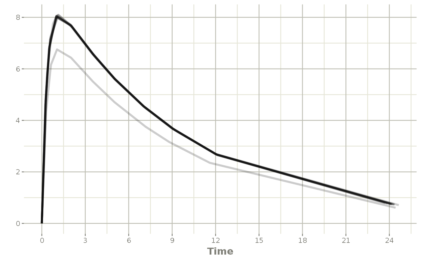
print(solveData)
#> ▂▂▂▂▂▂▂▂▂▂▂▂▂▂▂▂▂▂▂▂▂▂▂▂▂▂▂▂▂▂ Solved RxODE object ▂▂▂▂▂▂▂▂▂▂▂▂▂▂▂▂▂▂▂▂▂▂▂▂▂▂▂▂▂
#> ── Parameters ($params): ───────────────────────────────────────────────────────
#> # A tibble: 12 × 1
#>    id
#>    <fct>
#>  1 1
#>  2 2
#>  3 3
#>  4 4
#>  5 5
#>  6 6
#>  7 7
#>  8 8
#>  9 9
#> 10 10
#> 11 11
#> 12 12
#> ── Initial Conditions ($inits): ────────────────────────────────────────────────
#>  depot center
#>      0      0
#> ── First part of data (object): ────────────────────────────────────────────────
#> # A tibble: 132 × 8
#>      id  time    ka    cl     v    cp     depot center
#>   <int> <dbl> <dbl> <dbl> <dbl> <dbl>     <dbl>  <dbl>
#> 1     1  0     2.86  3.67  34.8  0    320.          0
#> 2     1  0.25  2.86  3.67  34.8  4.62 157.        161.
#> 3     1  0.57  2.86  3.67  34.8  7.12  62.8       248.
#> 4     1  1.12  2.86  3.67  34.8  8.09  13.0       282.
#> 5     1  2.02  2.86  3.67  34.8  7.68   0.996     267.
#> 6     1  3.82  2.86  3.67  34.8  6.38   0.00581   222.
#> # … with 126 more rows
#> ▂▂▂▂▂▂▂▂▂▂▂▂▂▂▂▂▂▂▂▂▂▂▂▂▂▂▂▂▂▂▂▂▂▂▂▂▂▂▂▂▂▂▂▂▂▂▂▂▂▂▂▂▂▂▂▂▂▂▂▂▂▂▂▂▂▂▂▂▂▂▂▂▂▂▂▂▂▂▂▂

## Of course the fasest way to solve if you don't care about the RxODE extra parameters is

solveData <- rxSolve(theo, parsDf, d, returnType="data.frame")

## solved data
dplyr::as.tbl(solveData)
#> Warning: `as.tbl()` was deprecated in dplyr 1.0.0.
#> Please use `tibble::as_tibble()` instead.
#> # A tibble: 132 × 8
#>       id  time    ka    cl     v    cp   depot center
#>    <int> <dbl> <dbl> <dbl> <dbl> <dbl>   <dbl>  <dbl>
#>  1     1  0     2.86  3.67  34.8  0    3.20e+2    0
#>  2     1  0.25  2.86  3.67  34.8  4.62 1.57e+2  161.
#>  3     1  0.57  2.86  3.67  34.8  7.12 6.28e+1  248.
#>  4     1  1.12  2.86  3.67  34.8  8.09 1.30e+1  282.
#>  5     1  2.02  2.86  3.67  34.8  7.68 9.96e-1  267.
#>  6     1  3.82  2.86  3.67  34.8  6.38 5.81e-3  222.
#>  7     1  5.1   2.86  3.67  34.8  5.58 1.50e-4  194.
#>  8     1  7.03  2.86  3.67  34.8  4.55 6.02e-7  158.
#>  9     1  9.05  2.86  3.67  34.8  3.68 1.77e-9  128.
#> 10     1 12.1   2.86  3.67  34.8  2.66 9.43e-9   92.6
#> # … with 122 more rows

data.table::data.table(solveData)
#>      id  time       ka       cl        v        cp         depot    center
#>   1:  1  0.00 2.857651 3.669297 34.81332 0.0000000  3.199920e+02   0.00000
#>   2:  1  0.25 2.857651 3.669297 34.81332 4.6240421  1.566295e+02 160.97825
#>   3:  1  0.57 2.857651 3.669297 34.81332 7.1151647  6.276731e+01 247.70249
#>   4:  1  1.12 2.857651 3.669297 34.81332 8.0922106  1.303613e+01 281.71670
#>   5:  1  2.02 2.857651 3.669297 34.81332 7.6837844  9.958446e-01 267.49803
#>  ---
#> 128: 12  5.07 2.857651 3.669297 34.81332 5.6044213  1.636210e-04 195.10850
#> 129: 12  7.07 2.857651 3.669297 34.81332 4.5392337  5.385697e-07 158.02579
#> 130: 12  9.03 2.857651 3.669297 34.81332 3.6920276  1.882087e-09 128.53173
#> 131: 12 12.05 2.857651 3.669297 34.81332 2.6855080  8.461424e-09  93.49144
#> 132: 12 24.15 2.857651 3.669297 34.81332 0.7501667 -4.775222e-10  26.11579