Event Table Function

Event Table Function

et(x, ..., envir = parent.frame())

# S3 method for RxODE
et(x, ..., envir = parent.frame())

# S3 method for rxSolve
et(x, ..., envir = parent.frame())

# S3 method for rxParams
et(x, ..., envir = parent.frame())

# S3 method for default
et(
  x,
  ...,
  time,
  amt,
  evid,
  cmt,
  ii,
  addl,
  ss,
  rate,
  dur,
  until,
  id,
  amountUnits,
  timeUnits,
  addSampling,
  envir = parent.frame(),
  by = NULL,
  length.out = NULL
)

Arguments

x	This is the first argument supplied to the event table. This is named to allow et to be used in a pipe-line with arbitrary objects.
...	Times or event tables. They can also be one of the named arguments below.
envir	the environment in which expr is to be evaluated. May also be NULL, a list, a data frame, a pairlist or an integer as specified to sys.call.
time	Time is the time of the dose or the sampling times. This can also be unspecified and is determined by the object type (list or numeric/integer).
amt	Amount of the dose. If specified, this assumes a dosing record, instead of a sampling record.
evid	Event ID; This can be: Numeric Value Description 0 An observation. This can also be specified as evid=obs 1 A dose observation. This can also be specified as evid=dose 2 A non-dose event. This can also be specified as evid=other 3 A reset event. This can also be specified as evid=reset. 4 Dose and reset event. This can also be specified as evid=doseReset or evid=resetDose Note a reset event resets all the compartment values to zero and turns off all infusions.
cmt	Compartment name or number. If a number, this is an integer starting at 1. Negative compartments turn off a compartment. If the compartment is a name, the compartment name is changed to the correct state/compartment number before running the simulation. For a compartment named "-cmt" the compartment is turned off. Can also specify `cmt` as `dosing.to`, `dose.to`, `doseTo`, `dosingTo`, and `state`.
ii	When specifying a dose, this is the inter-dose interval for ss, addl and until options (described below).
addl	The number of additional doses at a inter-dose interval after one dose.
ss	Steady state flag; It can be one of: Value Description 0 This dose is not a steady state dose 1 This dose is a steady state dose with the between/inter-dose interval of ii 2 Superposition steady state When ss=2 the steady state dose that uses the super-position principle to allow more complex steady states, like 10 mg in the morning and 20 mg at night, or dosing at 8 am 12 pm and 8 pm instead of every 12 hours. Since it uses the super positioning principle, it only makes sense when you know the kinetics are linear. All other values of SS are currently invalid.
rate	When positive, this is the rate of infusion. Otherwise: Value Description 0 No infusion is on this record -1 Modeled rate (in RxODE:rate(cmt) =); Can be et(rate=model). -2 Modeled duration (in RxODE: dur(cmt) =); Can beet(dur=model) or et(rate=dur). When a modeled bioavailability is applied to positive rates (rate > 0), the duration of infusion is changed. This is because the data specify the rate and amount, the only think that modeled bioavailability can affect is duration. If instead you want the modeled bioavailability to increase the rate of infusion instead of the duration of infusion, specify the dur instead or model the duration with rate=2.
dur	Duration of infusion. When amt and dur are specified the rate is calculated from the two data items. When dur is specified instead of rate, the bioavailability changes will increase rate instead of duration.
until	This is the time until the dosing should end. It can be an easier way to figure out how many additional doses are needed over your sampling period.
id	A integer vector of IDs to add or remove from the event table. If the event table is identical for each ID, then you may expand it to include all the IDs in this vector. All the negative IDs in this vector will be removed.
amountUnits	The units for the dosing records (amt)
timeUnits	The units for the time records (time)
addSampling	This is a boolean indicating if a sampling time should be added at the same time as a dosing time. By default this is FALSE.
by	When there are no observations in the event table, this is the amount to increment for the observations between from and to.
length.out	The number of observations to create if there isn't any observations in the event table. By default this is 200.

Value

A new event table

References

Wang W, Hallow K, James D (2015). "A Tutorial on RxODE: Simulating Differential Equation Pharmacometric Models in R." CPT: Pharmacometrics \& Systems Pharmacology, 5(1), 3-10. ISSN 2163-8306, <URL: https://www.ncbi.nlm.nih.gov/pmc/articles/PMC4728294/>.

See also

eventTable, add.sampling, add.dosing, et, etRep, etRbind, RxODE

Author

Matthew L Fidler, Wenping Wang

Examples

# \donttest{

library(RxODE)
library(units)

## Model from RxODE tutorial
mod1 <-RxODE({
    KA=2.94E-01;
    CL=1.86E+01;
    V2=4.02E+01;
    Q=1.05E+01;
    V3=2.97E+02;
    Kin=1;
    Kout=1;
    EC50=200;
    C2 = centr/V2;
    C3 = peri/V3;
    d/dt(depot) =-KA*depot;
    d/dt(centr) = KA*depot - CL*C2 - Q*C2 + Q*C3;
    d/dt(peri)  =                    Q*C2 - Q*C3;
    d/dt(eff)  = Kin - Kout*(1-C2/(EC50+C2))*eff;
});
#>  

## These are making the more complex regimens of the RxODE tutorial

## bid for 5 days
bid <- et(timeUnits="hr") %>%
       et(amt=10000,ii=12,until=set_units(5, "days"))

## qd for 5 days
qd <- et(timeUnits="hr") %>%
      et(amt=20000,ii=24,until=set_units(5, "days"))

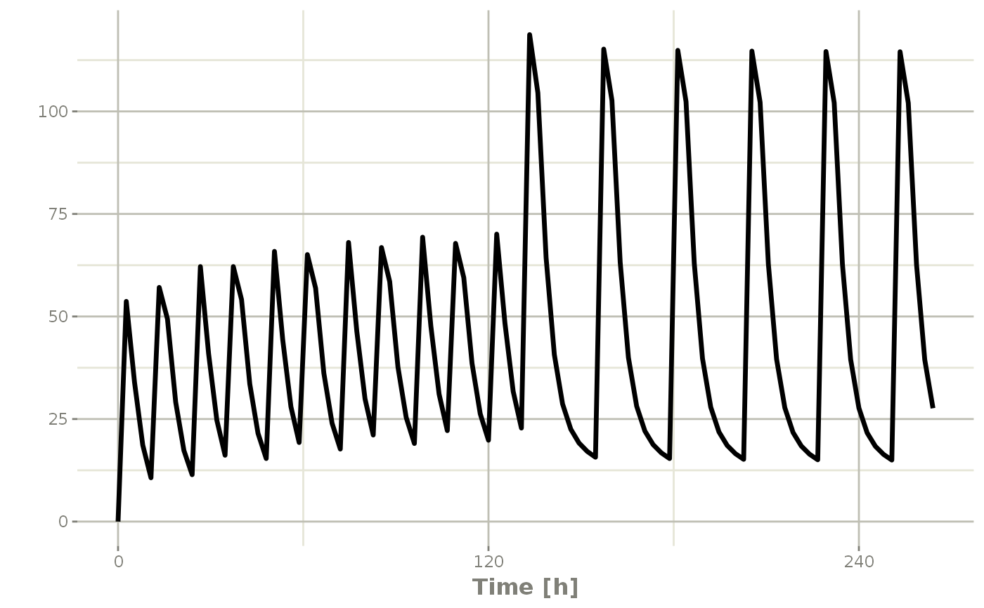
## bid for 5 days followed by qd for 5 days

et <- seq(bid,qd) %>% et(seq(0,11*24,length.out=100));

bidQd <- rxSolve(mod1, et)

plot(bidQd, C2)



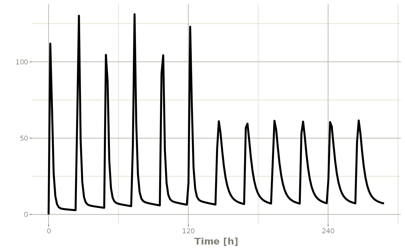
## Now Infusion for 5 days followed by oral for 5 days

##  note you can dose to a named compartment instead of using the compartment number
infusion <- et(timeUnits = "hr") %>%
      et(amt=10000, rate=5000, ii=24, until=set_units(5, "days"), cmt="centr")


qd <- et(timeUnits = "hr") %>% et(amt=10000, ii=24, until=set_units(5, "days"), cmt="depot")

et <- seq(infusion,qd)

infusionQd <- rxSolve(mod1, et)

plot(infusionQd, C2)


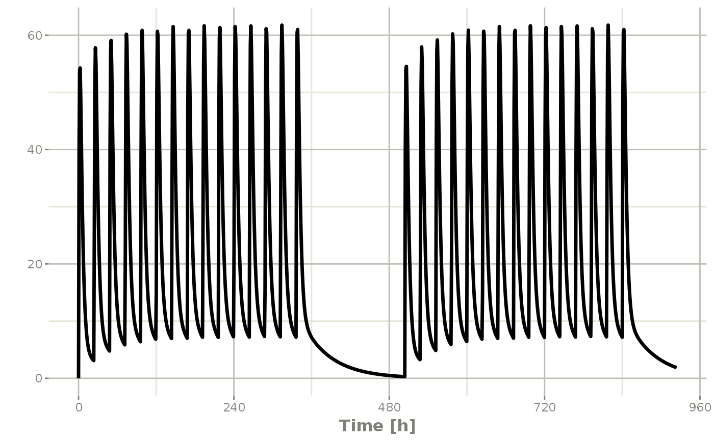
## 2wk-on, 1wk-off

qd <- et(timeUnits = "hr") %>% et(amt=10000, ii=24, until=set_units(2, "weeks"), cmt="depot")

et <- seq(qd, set_units(1,"weeks"), qd) %>%
     add.sampling(set_units(seq(0, 5.5,by=0.005),weeks))

wkOnOff <- rxSolve(mod1, et)

plot(wkOnOff, C2)


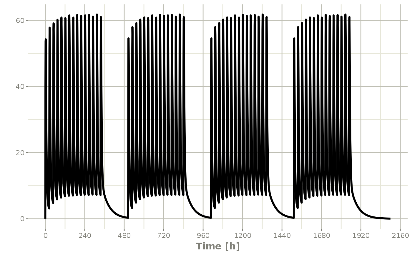
## You can also repeat the cycle easily with the rep function

qd <-et(timeUnits = "hr") %>% et(amt=10000, ii=24, until=set_units(2, "weeks"), cmt="depot")

et <- etRep(qd, times=4, wait=set_units(1,"weeks")) %>%
     add.sampling(set_units(seq(0, 12.5,by=0.005),weeks))

repCycle4 <- rxSolve(mod1, et)

plot(repCycle4, C2)


# }