Combining event tables

etRbind(
  ...,
  samples = c("use", "clear"),
  waitII = c("smart", "+ii"),
  id = c("merge", "unique")
)

# S3 method for rxEt
rbind(..., deparse.level = 1)

Arguments

...	The event tables and optionally time between event tables, called waiting times in this help document.
samples	How to handle samples when repeating an event table. The options are: `"clear"` Clear sampling records before combining the datasets `"use"` Use the sampling records when combining the datasets
waitII	This determines how waiting times between events are handled. The options are: `"smart"` This "smart" handling of waiting times is the default option. In this case, if the waiting time is above the last observed inter-dose interval in the first combined event table, then the actual time between doses is given by the wait time. If it is smaller than the last observed inter-dose interval, the time between event tables is given by the inter-dose interval + the waiting time between event tables. `"+ii"` In this case, the wait time is added to the inter-dose interval no matter the length of the wait time or inter-dose interval
id	This is how rbind will handle IDs. There are two different types of options: `merge` with `id="merge"`, the IDs are merged together, overlapping IDs would be merged into a single event table. `unique` with `id="unique"`, the IDs will be renumbered so that the IDs in all the event tables are not overlapping.
deparse.level	The `deparse.level` of a traditional `rbind` is ignored.

Value

An event table

References

Wang W, Hallow K, James D (2015). "A Tutorial on RxODE: Simulating Differential Equation Pharmacometric Models in R." CPT: Pharmacometrics \& Systems Pharmacology, 5(1), 3-10. ISSN 2163-8306, <URL: https://www.ncbi.nlm.nih.gov/pmc/articles/PMC4728294/>.

Author

Matthew L Fidler

Matthew L Fidler, Wenping Wang

Examples


# \donttest{

library(RxODE)
library(units)

## Model from RxODE tutorial
mod1 <-RxODE({
    KA=2.94E-01;
    CL=1.86E+01;
    V2=4.02E+01;
    Q=1.05E+01;
    V3=2.97E+02;
    Kin=1;
    Kout=1;
    EC50=200;
    C2 = centr/V2;
    C3 = peri/V3;
    d/dt(depot) =-KA*depot;
    d/dt(centr) = KA*depot - CL*C2 - Q*C2 + Q*C3;
    d/dt(peri)  =                    Q*C2 - Q*C3;
    d/dt(eff)  = Kin - Kout*(1-C2/(EC50+C2))*eff;
});
#>  

## These are making the more complex regimens of the RxODE tutorial

## bid for 5 days
bid <- et(timeUnits="hr") %>%
       et(amt=10000,ii=12,until=set_units(5, "days"))

## qd for 5 days
qd <- et(timeUnits="hr") %>%
      et(amt=20000,ii=24,until=set_units(5, "days"))

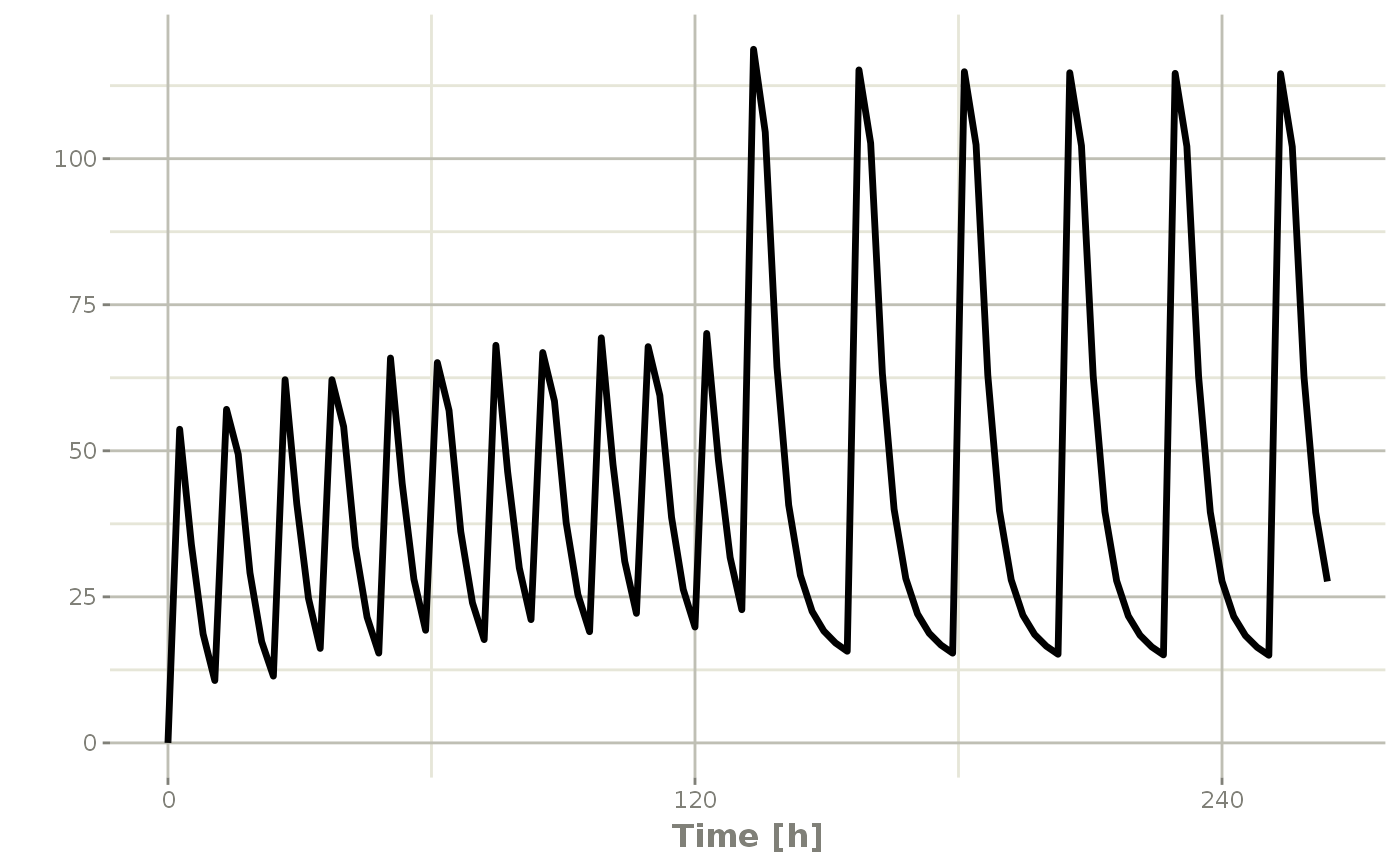
## bid for 5 days followed by qd for 5 days

et <- seq(bid,qd) %>% et(seq(0,11*24,length.out=100));

bidQd <- rxSolve(mod1, et)

plot(bidQd, C2)



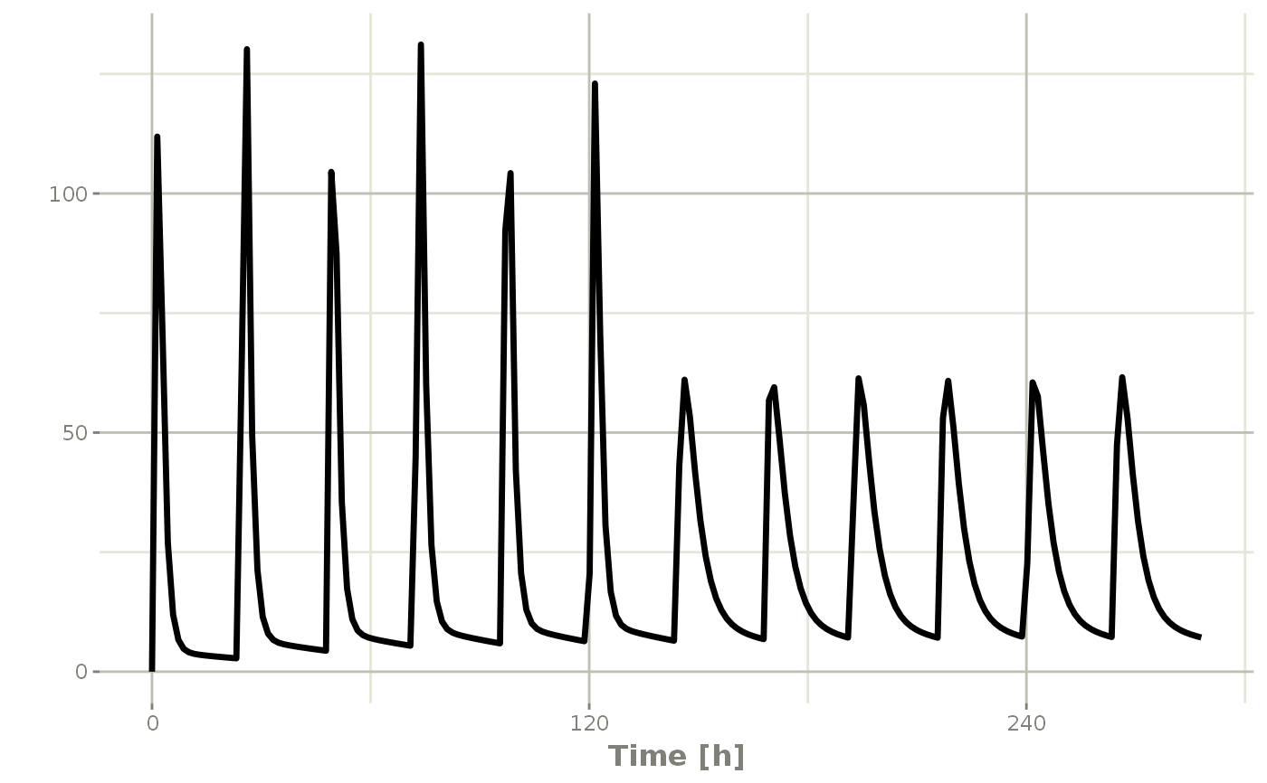
## Now Infusion for 5 days followed by oral for 5 days

##  note you can dose to a named compartment instead of using the compartment number
infusion <- et(timeUnits = "hr") %>%
      et(amt=10000, rate=5000, ii=24, until=set_units(5, "days"), cmt="centr")


qd <- et(timeUnits = "hr") %>% et(amt=10000, ii=24, until=set_units(5, "days"), cmt="depot")

et <- seq(infusion,qd)

infusionQd <- rxSolve(mod1, et)

plot(infusionQd, C2)


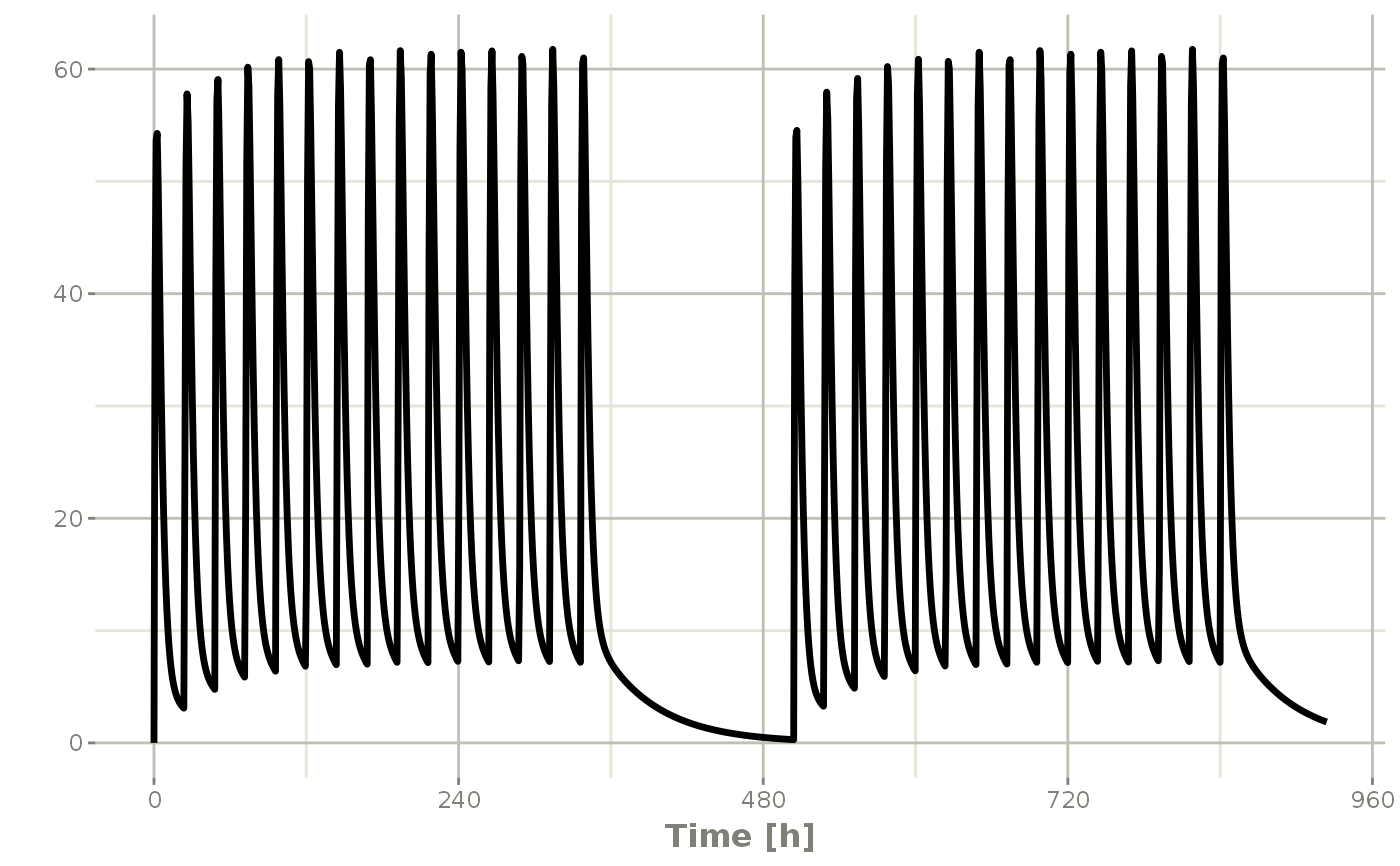
## 2wk-on, 1wk-off

qd <- et(timeUnits = "hr") %>% et(amt=10000, ii=24, until=set_units(2, "weeks"), cmt="depot")

et <- seq(qd, set_units(1,"weeks"), qd) %>%
     add.sampling(set_units(seq(0, 5.5,by=0.005),weeks))

wkOnOff <- rxSolve(mod1, et)

plot(wkOnOff, C2)


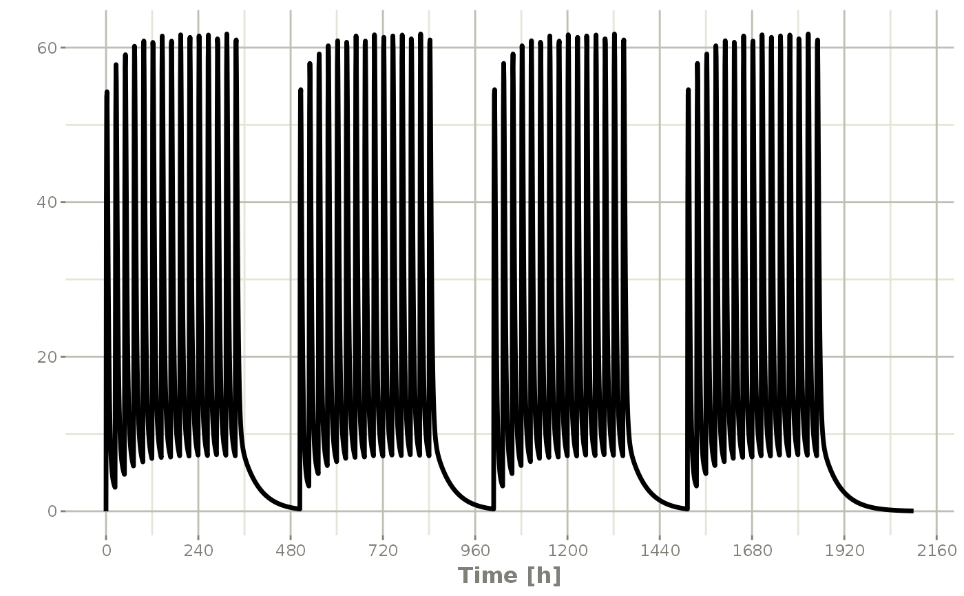
## You can also repeat the cycle easily with the rep function

qd <-et(timeUnits = "hr") %>% et(amt=10000, ii=24, until=set_units(2, "weeks"), cmt="depot")

et <- etRep(qd, times=4, wait=set_units(1,"weeks")) %>%
     add.sampling(set_units(seq(0, 12.5,by=0.005),weeks))

repCycle4 <- rxSolve(mod1, et)

plot(repCycle4, C2)


# }