Friberg Myelosuppression model


library(nlmixr)
library(xpose)
library(xpose.nlmixr)


wbc <- function() {
  ini({
    ## Note that the UI can take expressions
    ## Also note that these initial estimates should be provided on the log-scale
    log_CIRC0 <- log(7.21)
    log_MTT <- log(124)
    log_SLOPU <- log(28.9)
    log_GAMMA <- log(0.239)
    ## Initial estimates should be high for SAEM ETAs
    eta.CIRC0  ~ .1
    eta.MTT  ~ .03
    eta.SLOPU ~ .2
    ##  Also true for additive error (also ignored in SAEM)
    prop.err <- 10
  })
  model({
    CIRC0 =  exp(log_CIRC0 + eta.CIRC0)
    MTT =  exp(log_MTT + eta.MTT)
    SLOPU =  exp(log_SLOPU + eta.SLOPU)
    GAMMA = exp(log_GAMMA)

    # PK parameters from input dataset
    CL = CLI;
    V1 = V1I;
    V2 = V2I;
    Q = 204;

    CONC = A_centr/V1;

    # PD parameters
    NN = 3;
    KTR = (NN + 1)/MTT;
    EDRUG = 1 - SLOPU * CONC;
    FDBK = (CIRC0 / A_circ)^GAMMA;

    CIRC = A_circ;

    A_prol(0) = CIRC0;
    A_tr1(0) = CIRC0;
    A_tr2(0) = CIRC0;
    A_tr3(0) = CIRC0;
    A_circ(0) = CIRC0;

    d/dt(A_centr) = A_periph * Q/V2 - A_centr * (CL/V1 + Q/V1);
    d/dt(A_periph) = A_centr * Q/V1 - A_periph * Q/V2;
    d/dt(A_prol) = KTR * A_prol * EDRUG * FDBK - KTR * A_prol;
    d/dt(A_tr1) = KTR * A_prol - KTR * A_tr1;
    d/dt(A_tr2) = KTR * A_tr1 - KTR * A_tr2;
    d/dt(A_tr3) = KTR * A_tr2 - KTR * A_tr3;
    d/dt(A_circ) = KTR * A_tr3 - KTR * A_circ;

    CIRC ~ prop(prop.err)
  })
}

Fit model using saem

d3 = read.csv("Simulated_WBC_pacl_ddmore_samePK_nlmixr.csv", na.string = ".")

fit.S <- nlmixr(wbc, d3, est="saem", list(print=0), table=list(cwres=TRUE, npde=TRUE))
#> [====|====|====|====|====|====|====|====|====|====] 0:00:00 
#> 
#> [====|====|====|====|====|====|====|====|====|====] 0:00:00 
#> 
#> [====|====|====|====|====|====|====|====|====|====] 0:00:00 
#> 
#> [====|====|====|====|====|====|====|====|====|====] 0:00:00 
#> 
#> [====|====|====|====|====|====|====|====|====|====] 0:00:00 
#> 
#> [1] "V2I" "CLI" "V1I"
#> [====|====|====|====|====|====|====|====|====|====] 0:00:04

xpdb <- xpose_data_nlmixr(fit.S)
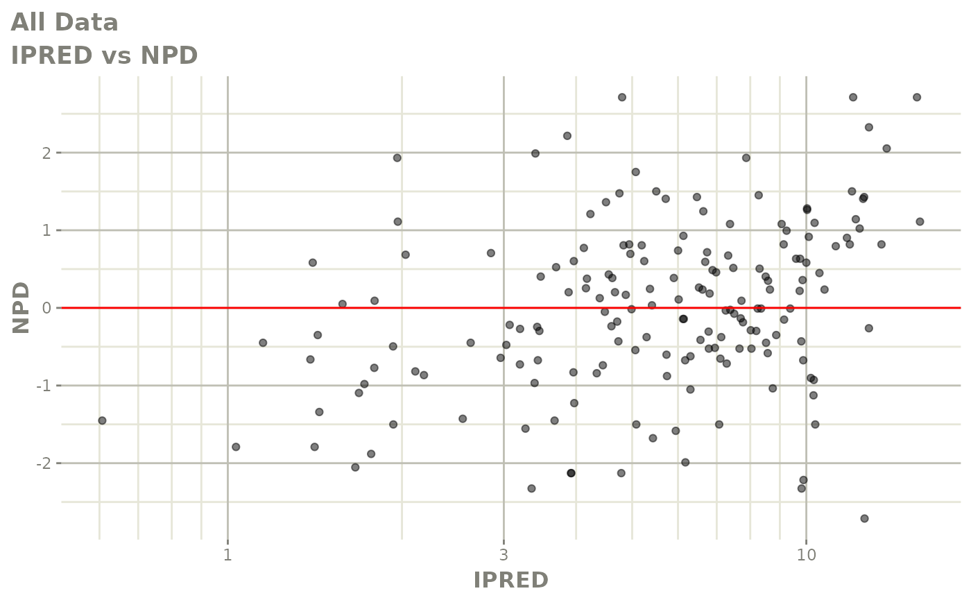
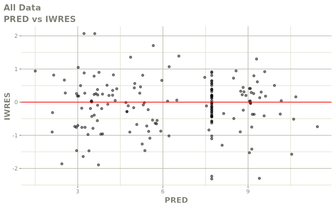
plot(fit.S)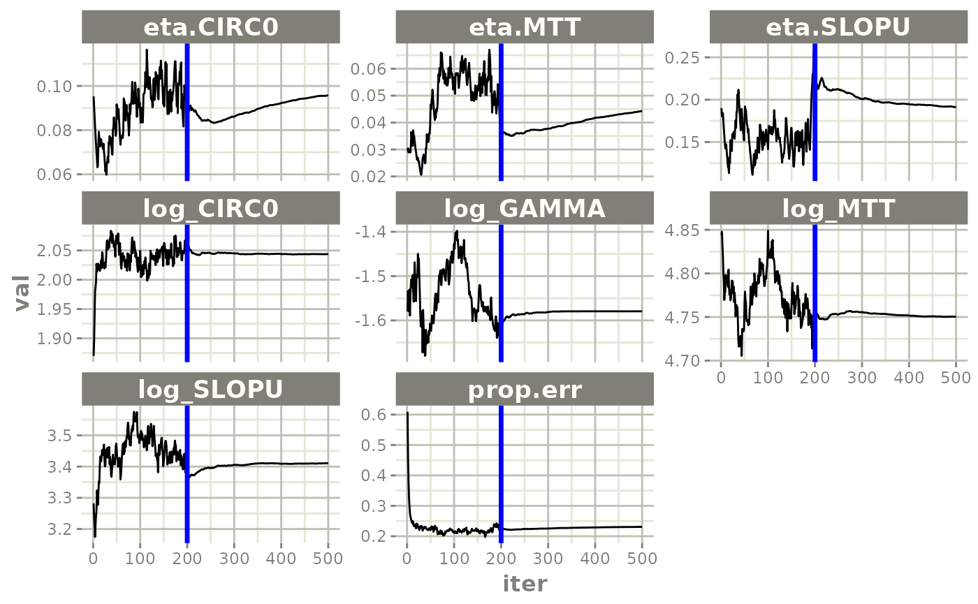

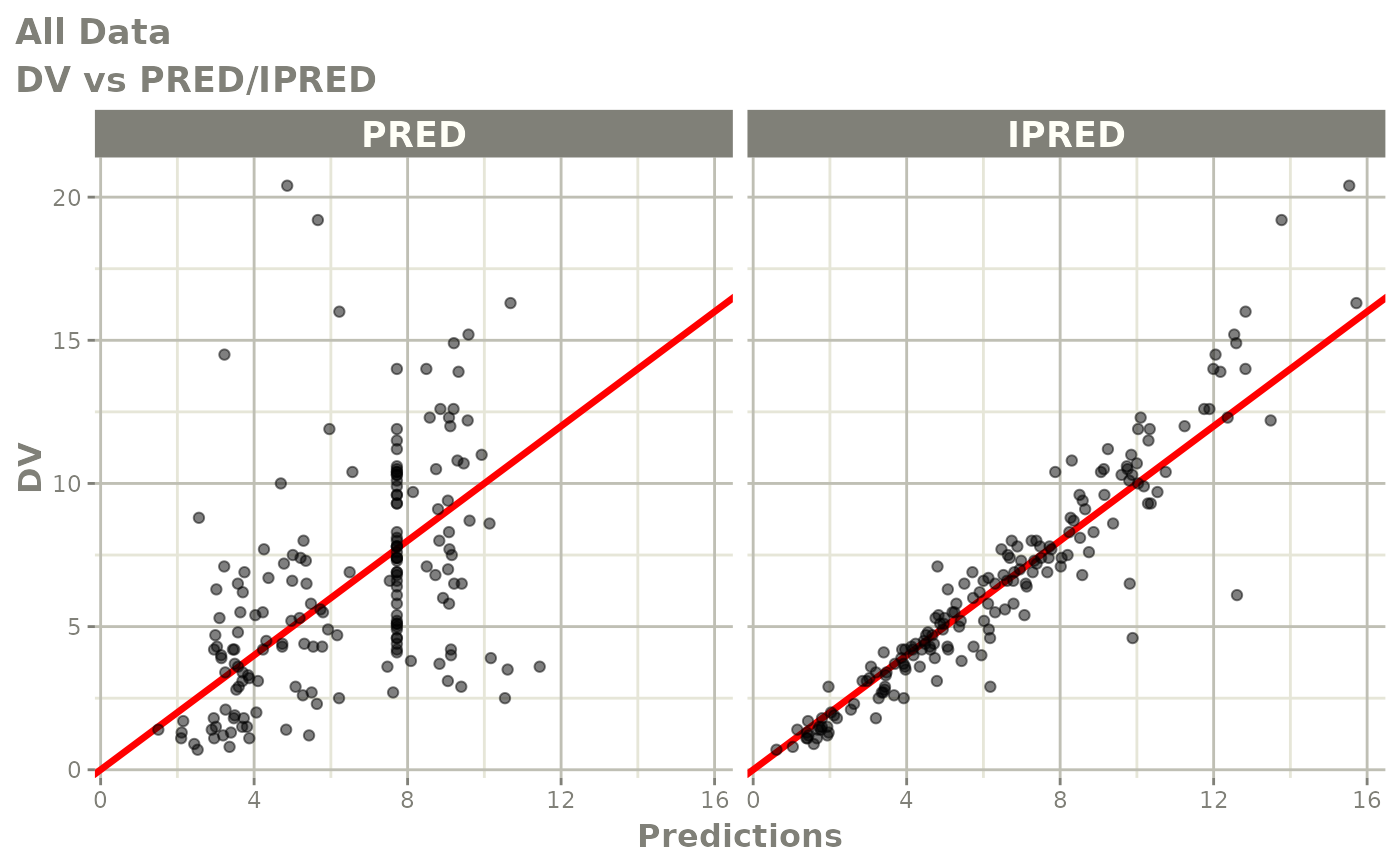
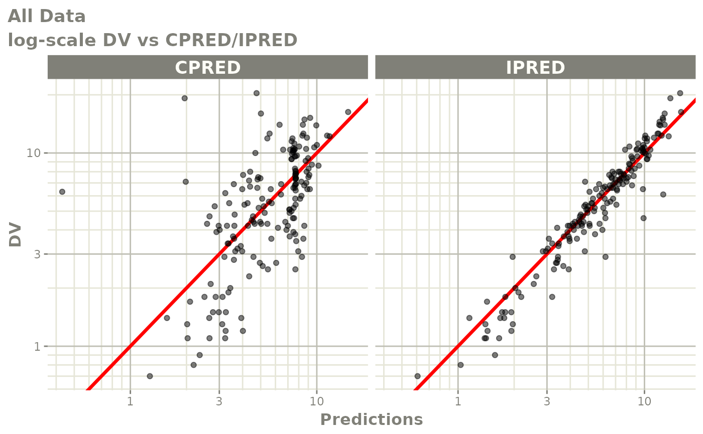
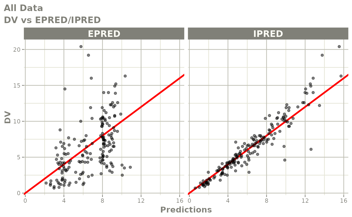
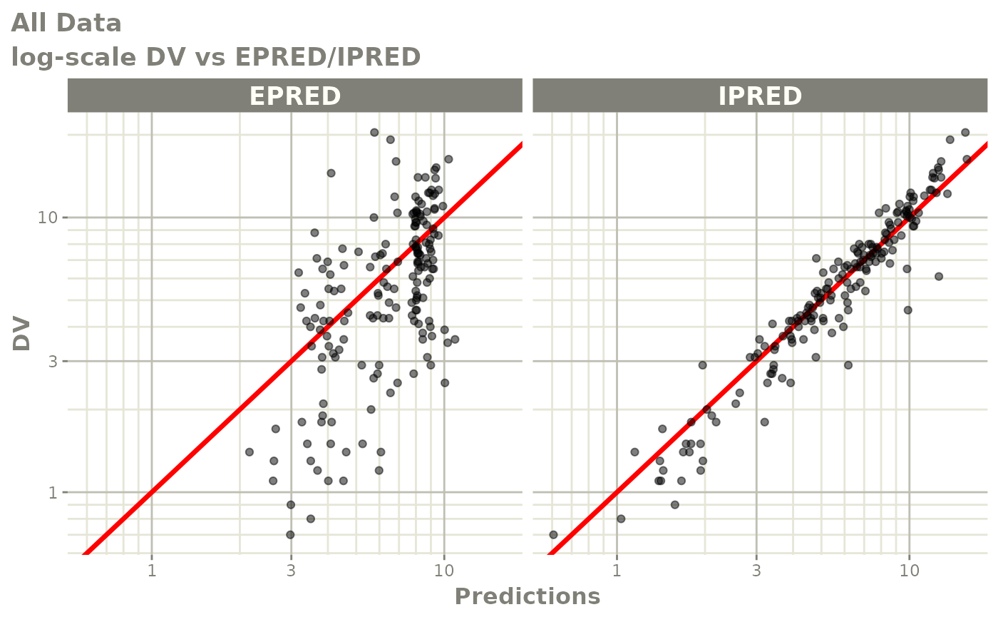
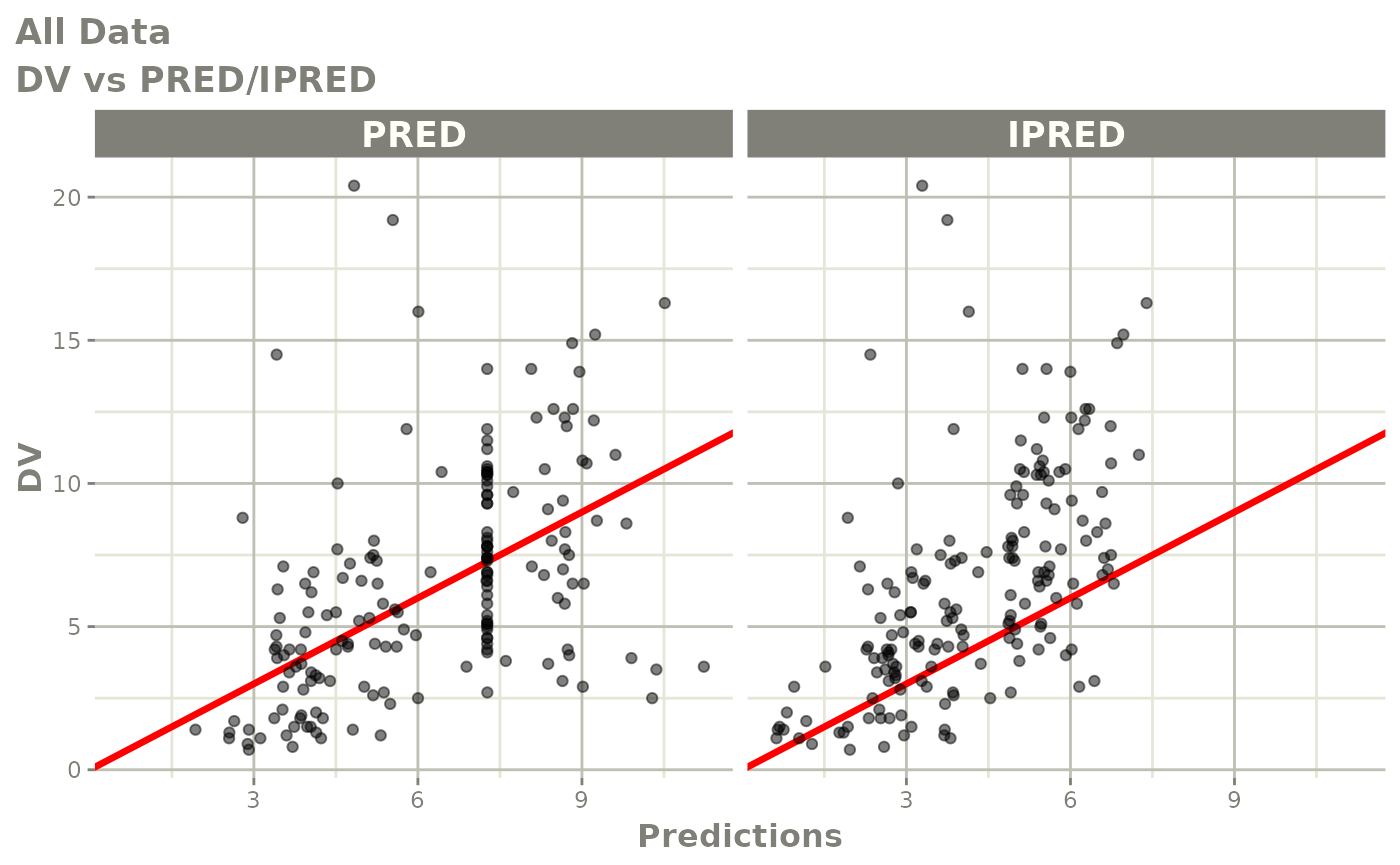
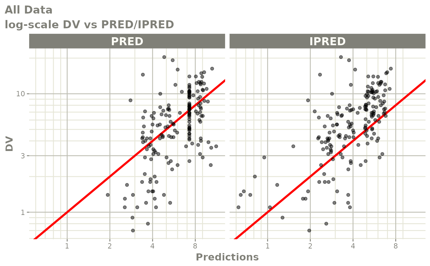
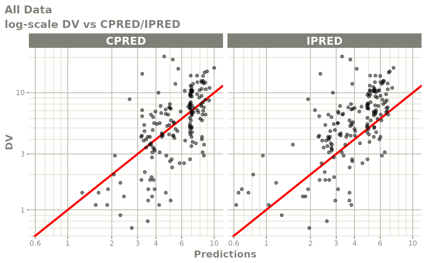
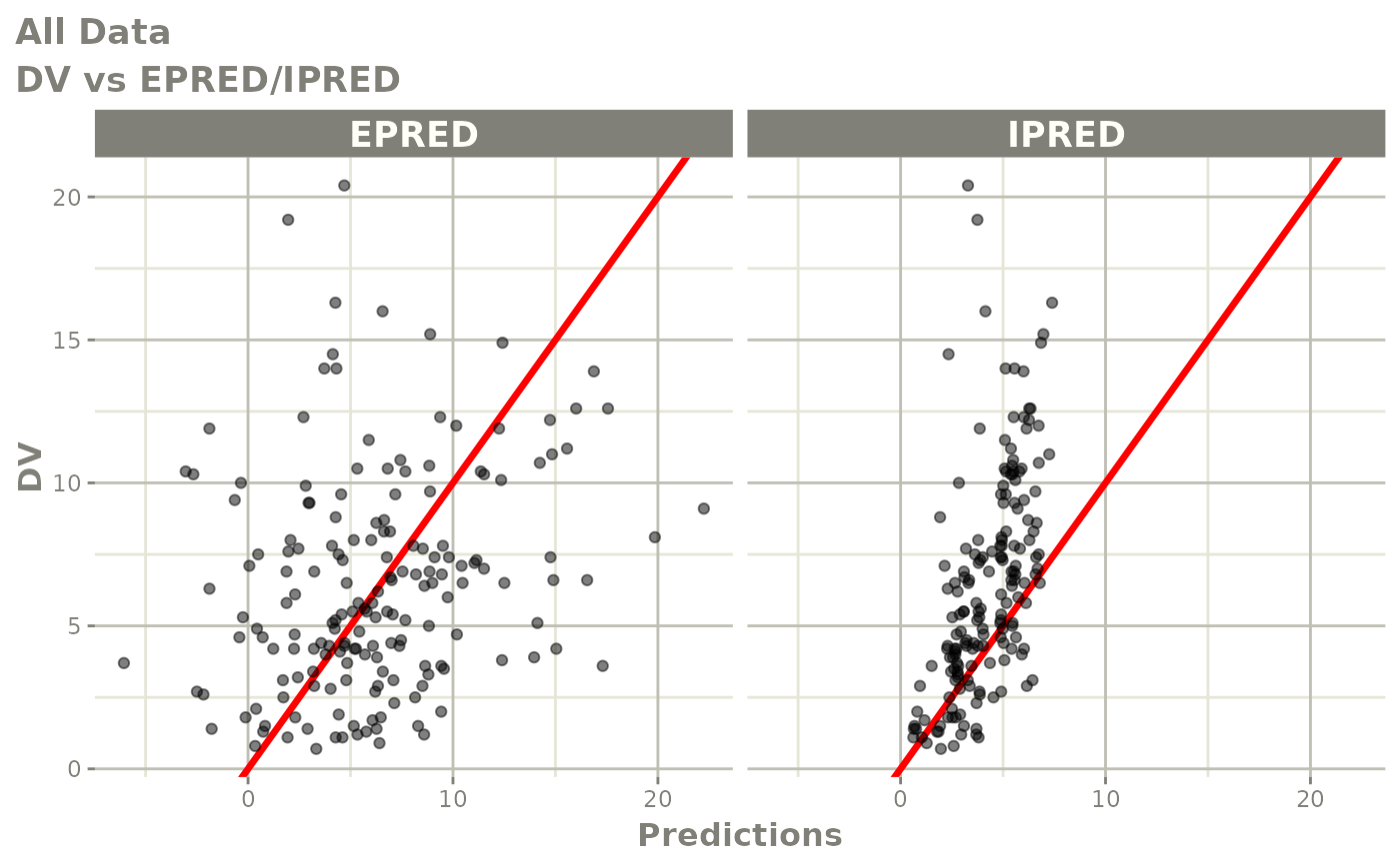
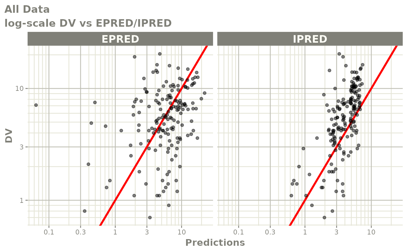
print(dv_vs_pred(xpdb) +
      ylab("Observed Neutrophil Count (10^9/L)") +
      xlab("Population Predicted Neutrophil Count (10^9/L)"))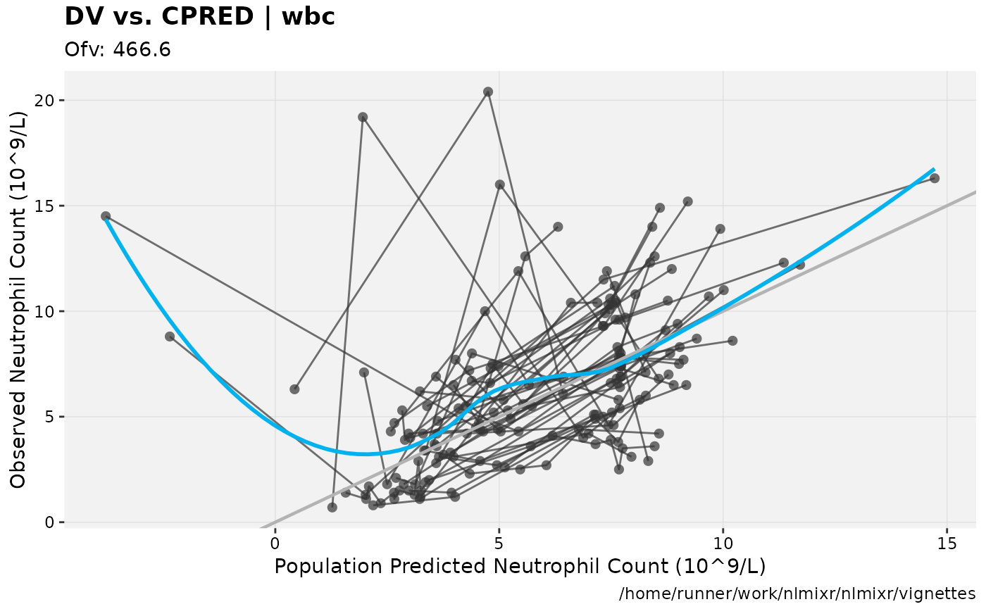


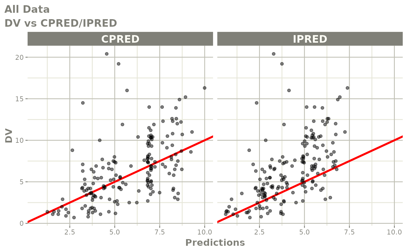
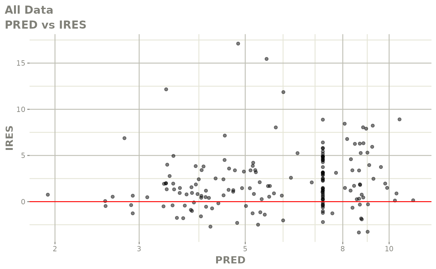
print(dv_vs_ipred(xpdb) +
      ylab("Observed Neutrophil Count (10^9/L)") +
      xlab("Individual Predicted Neutrophil Count (10^9/L)"))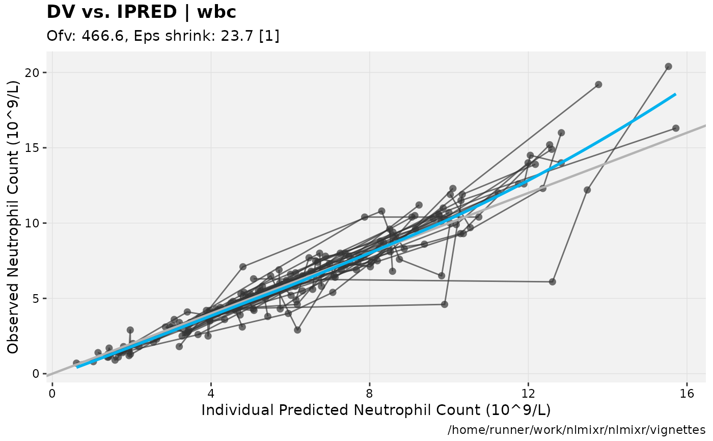


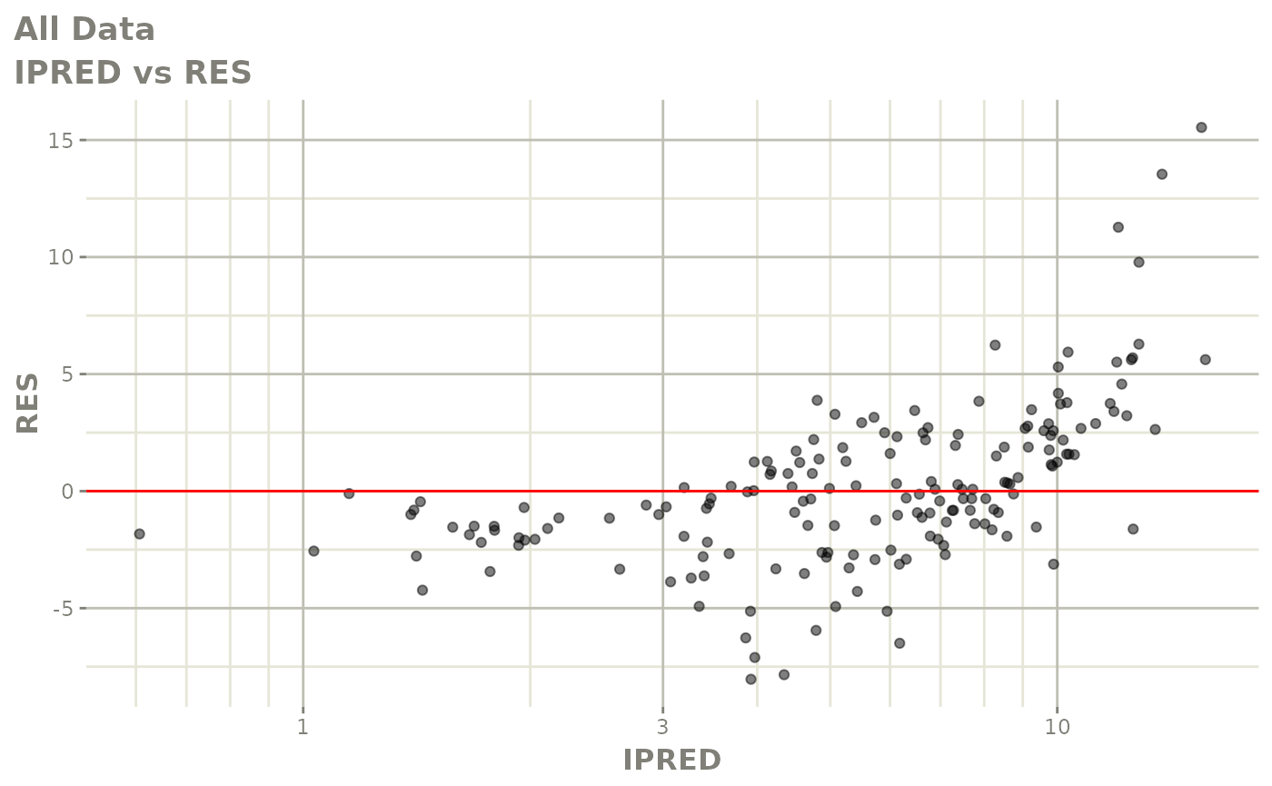
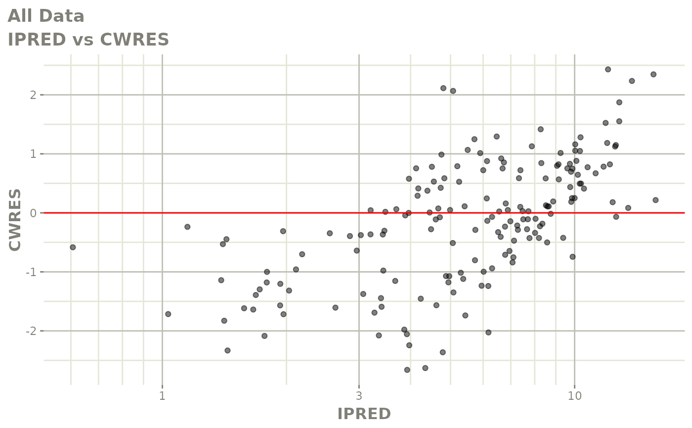
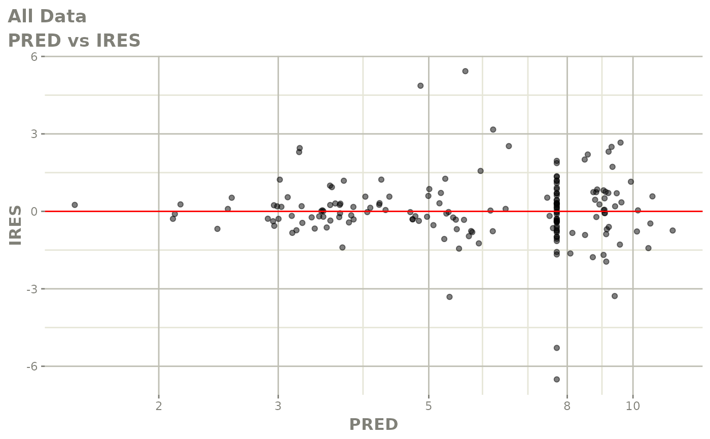
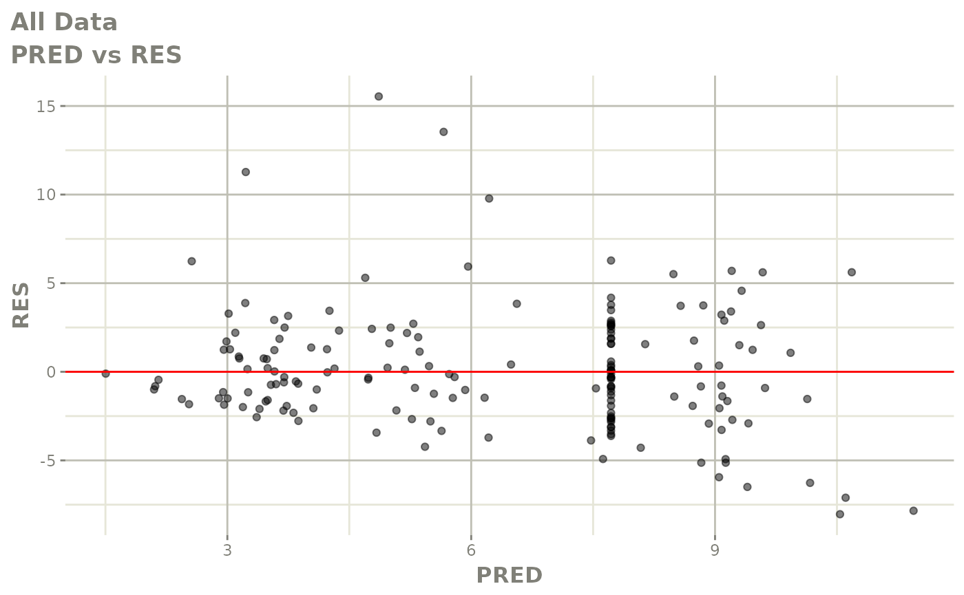
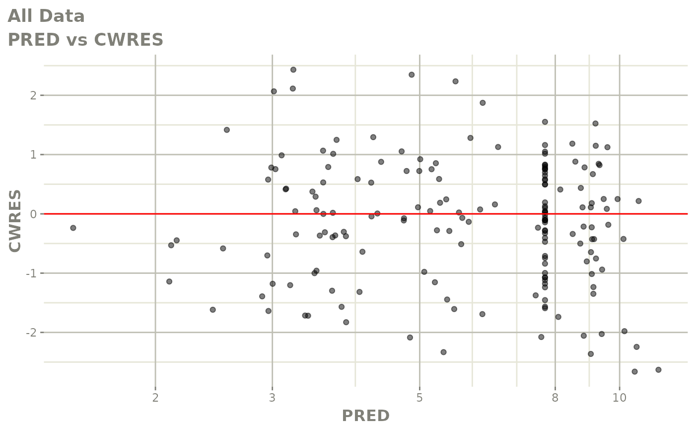
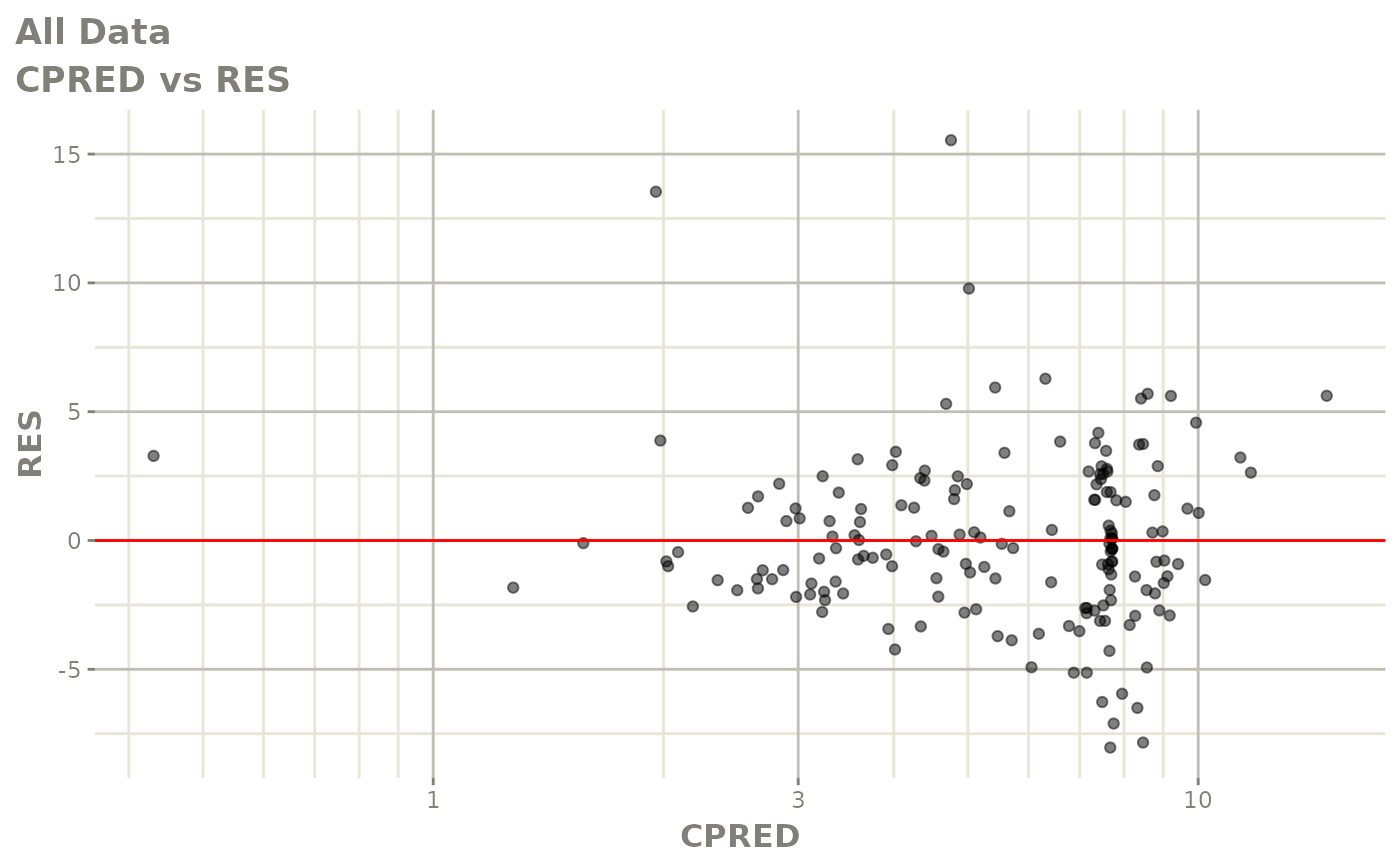
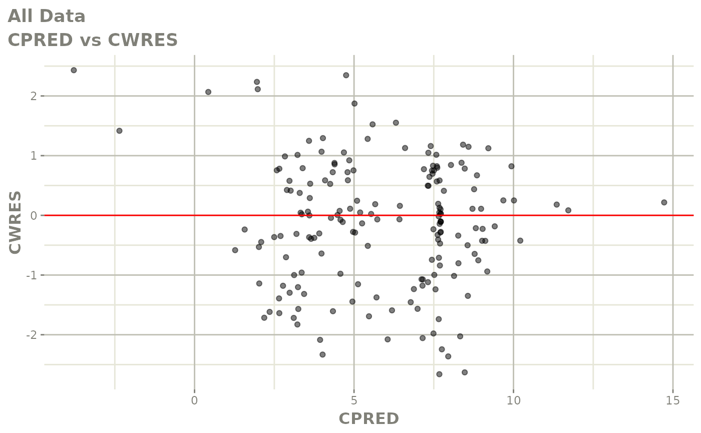
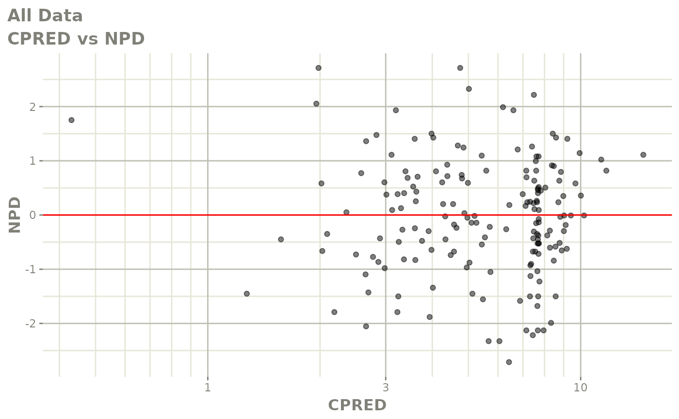
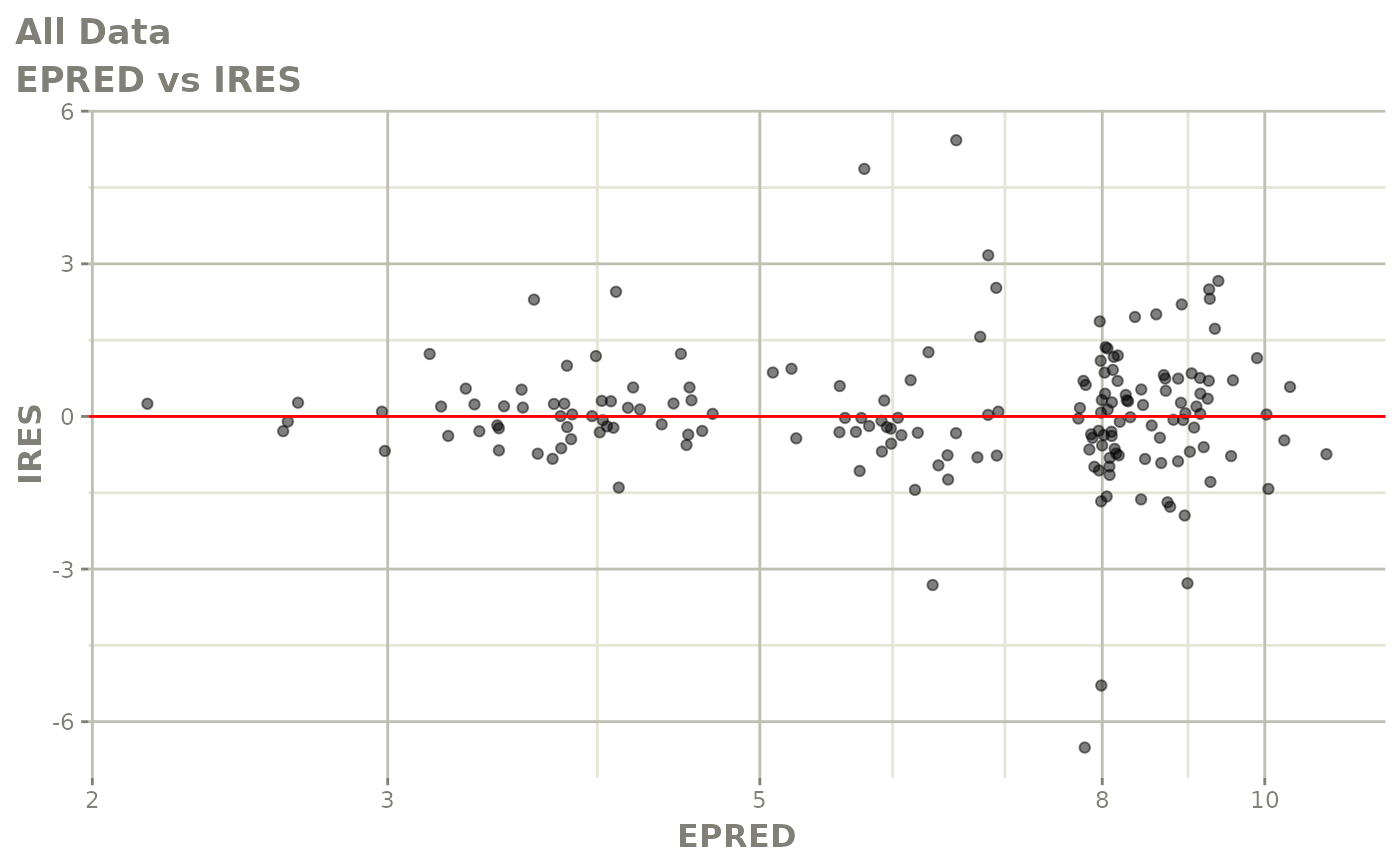
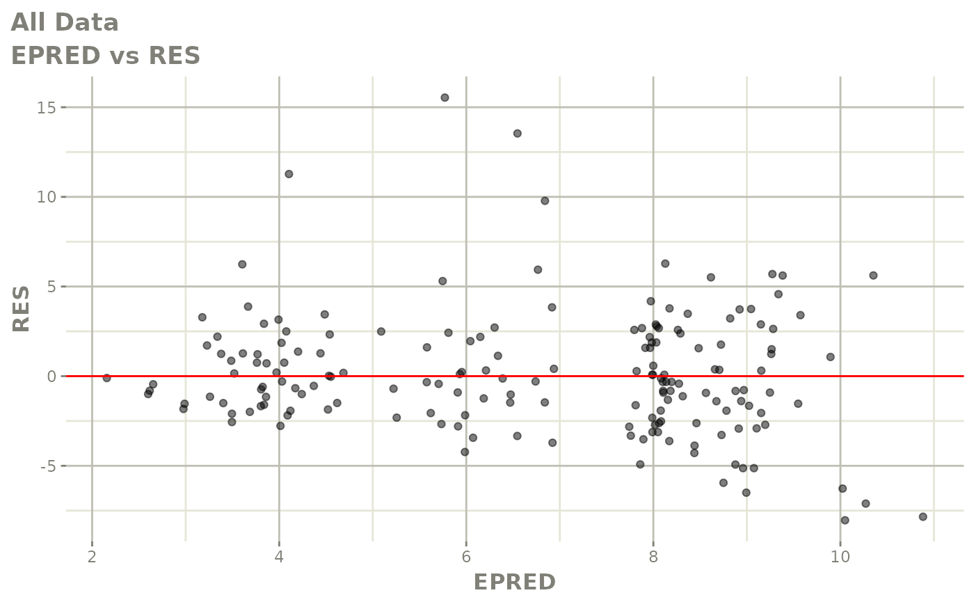
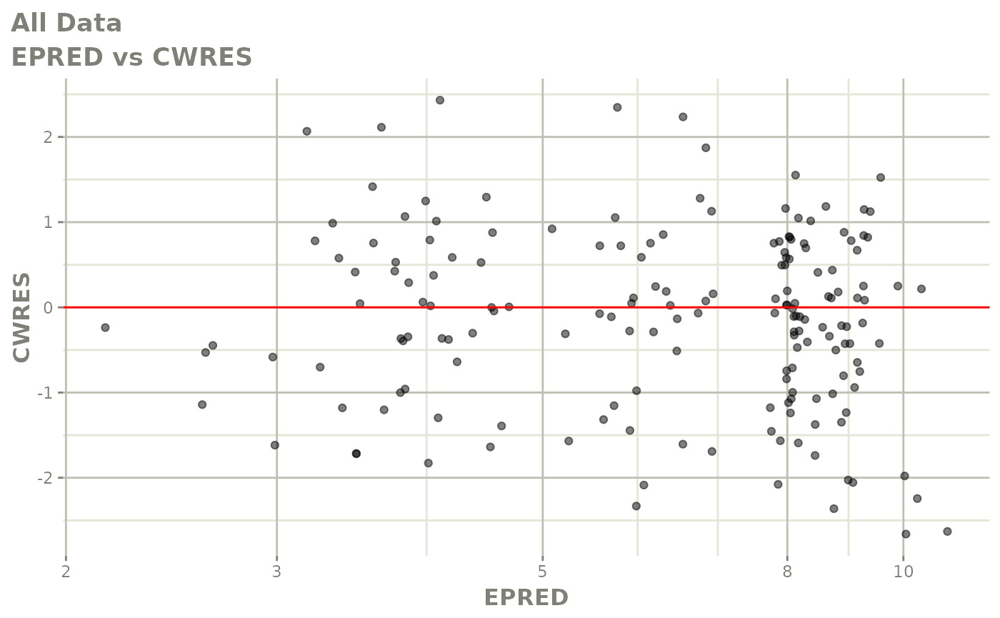
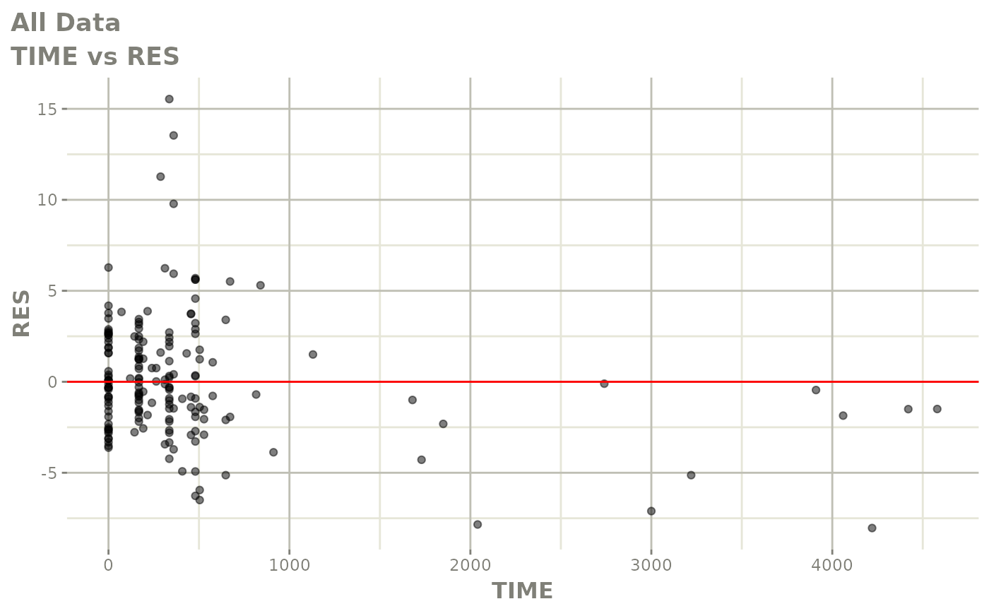
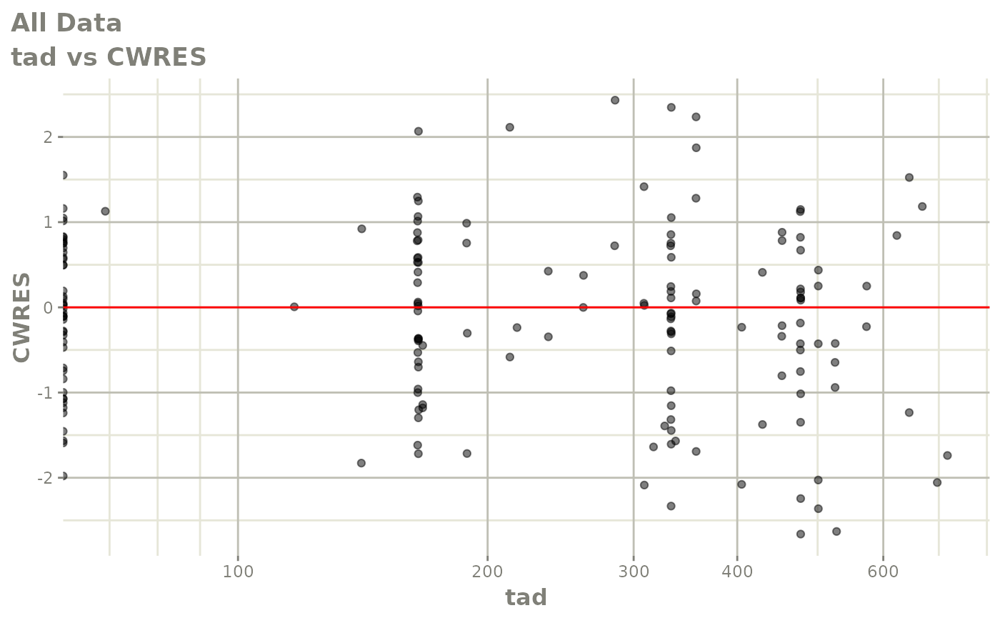
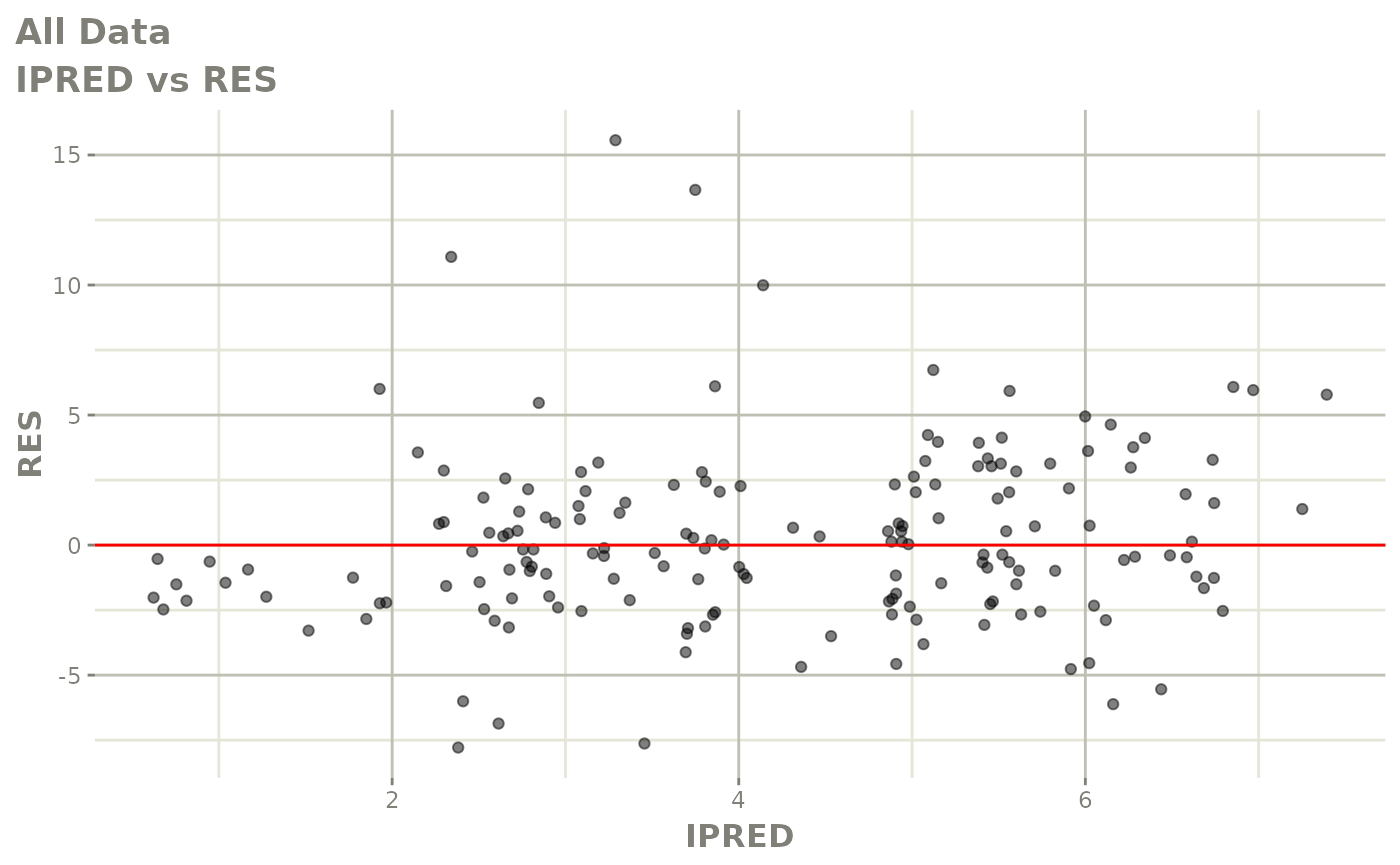
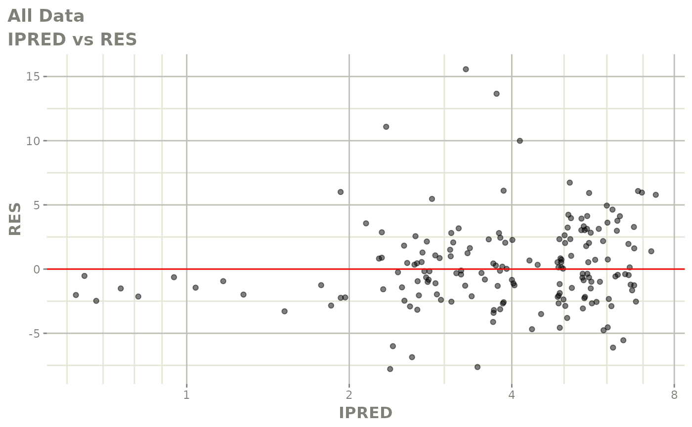
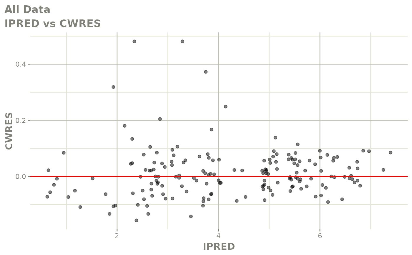
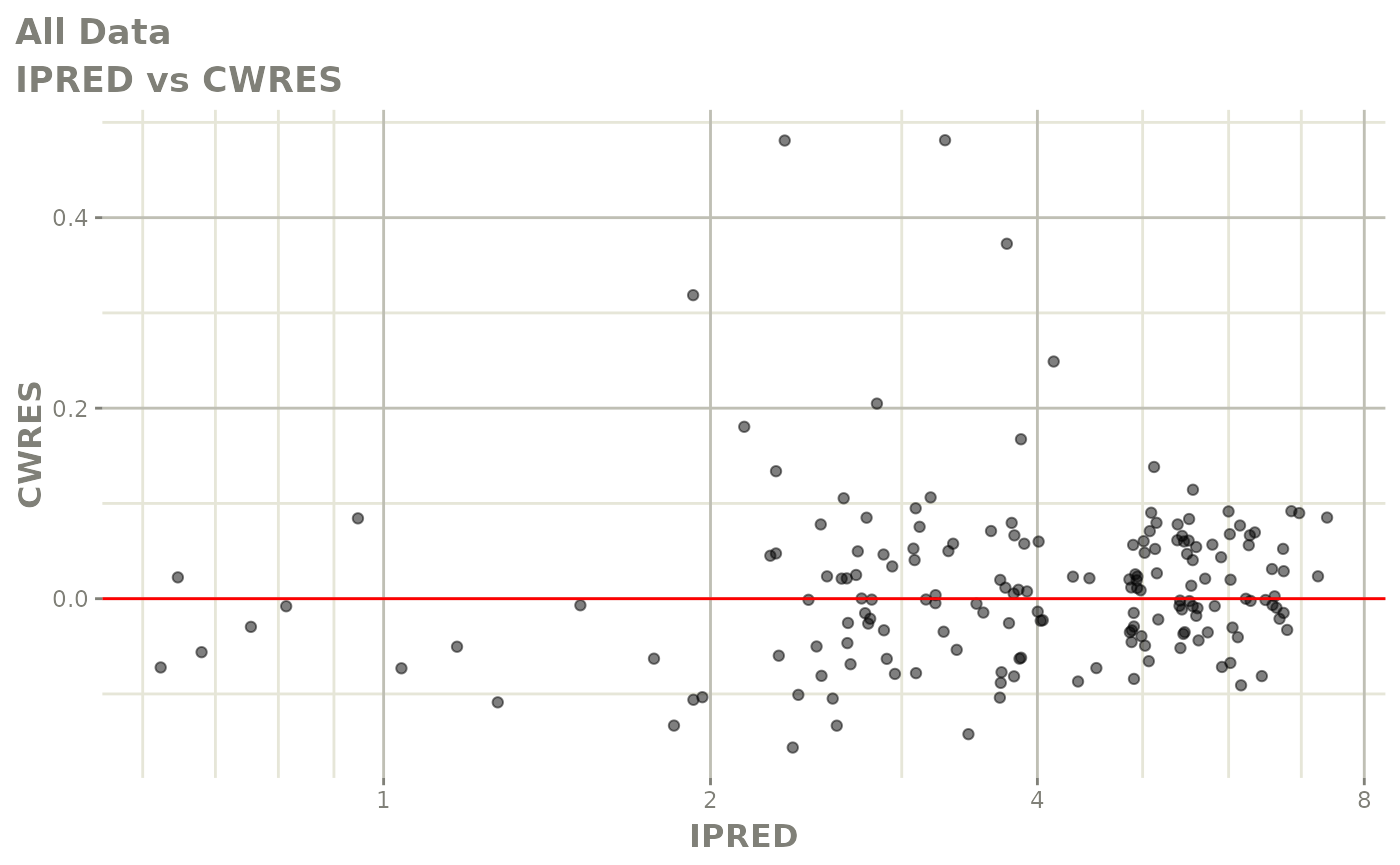
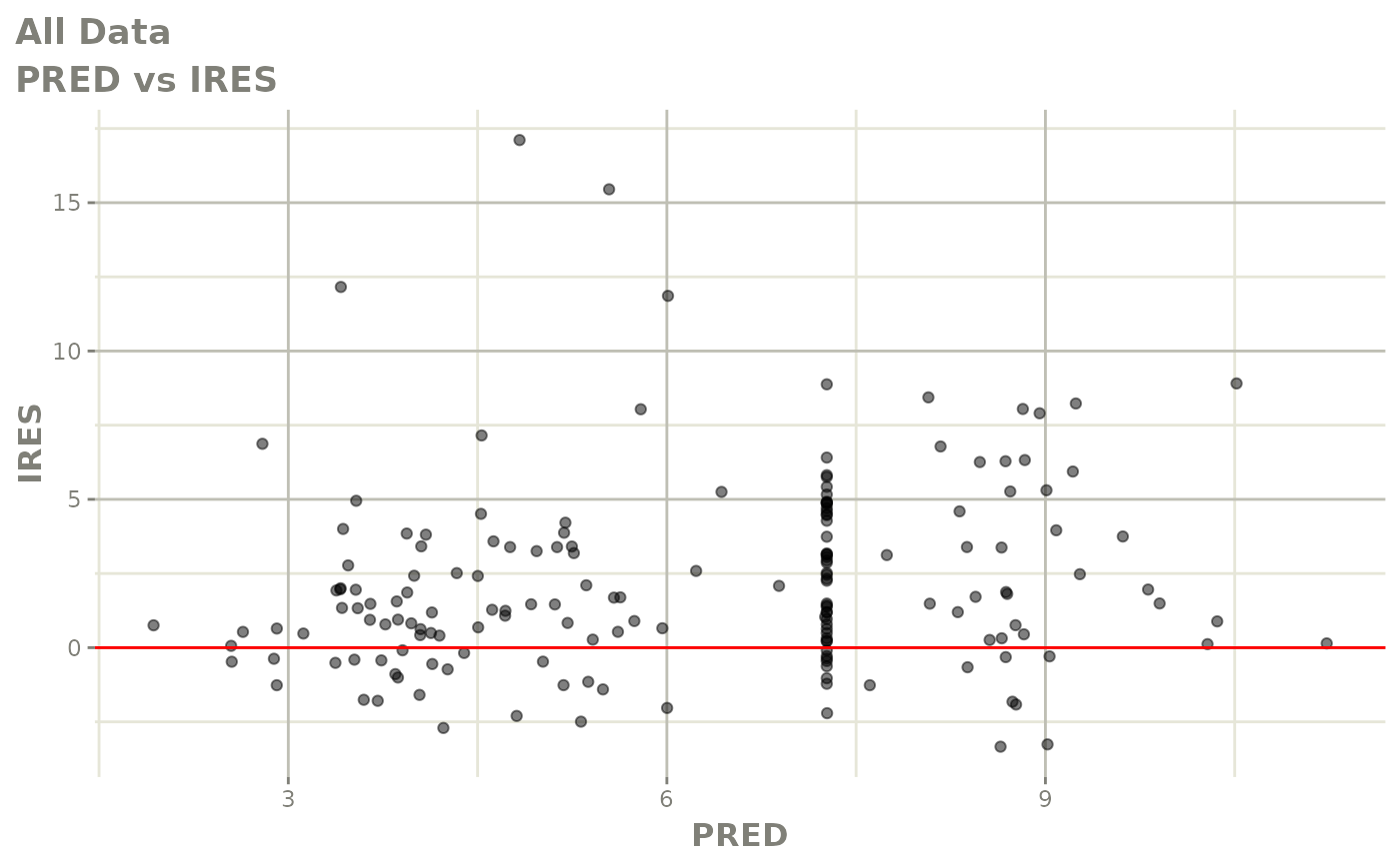
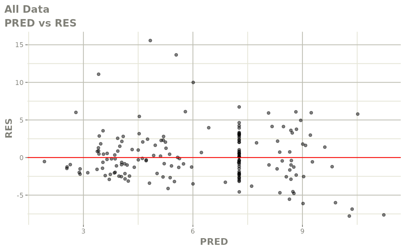
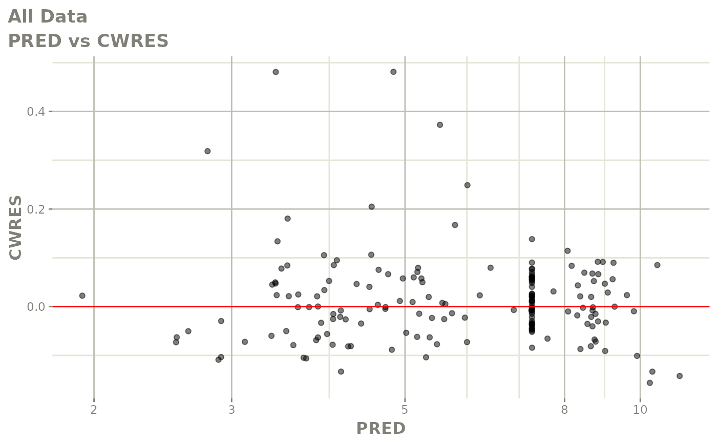
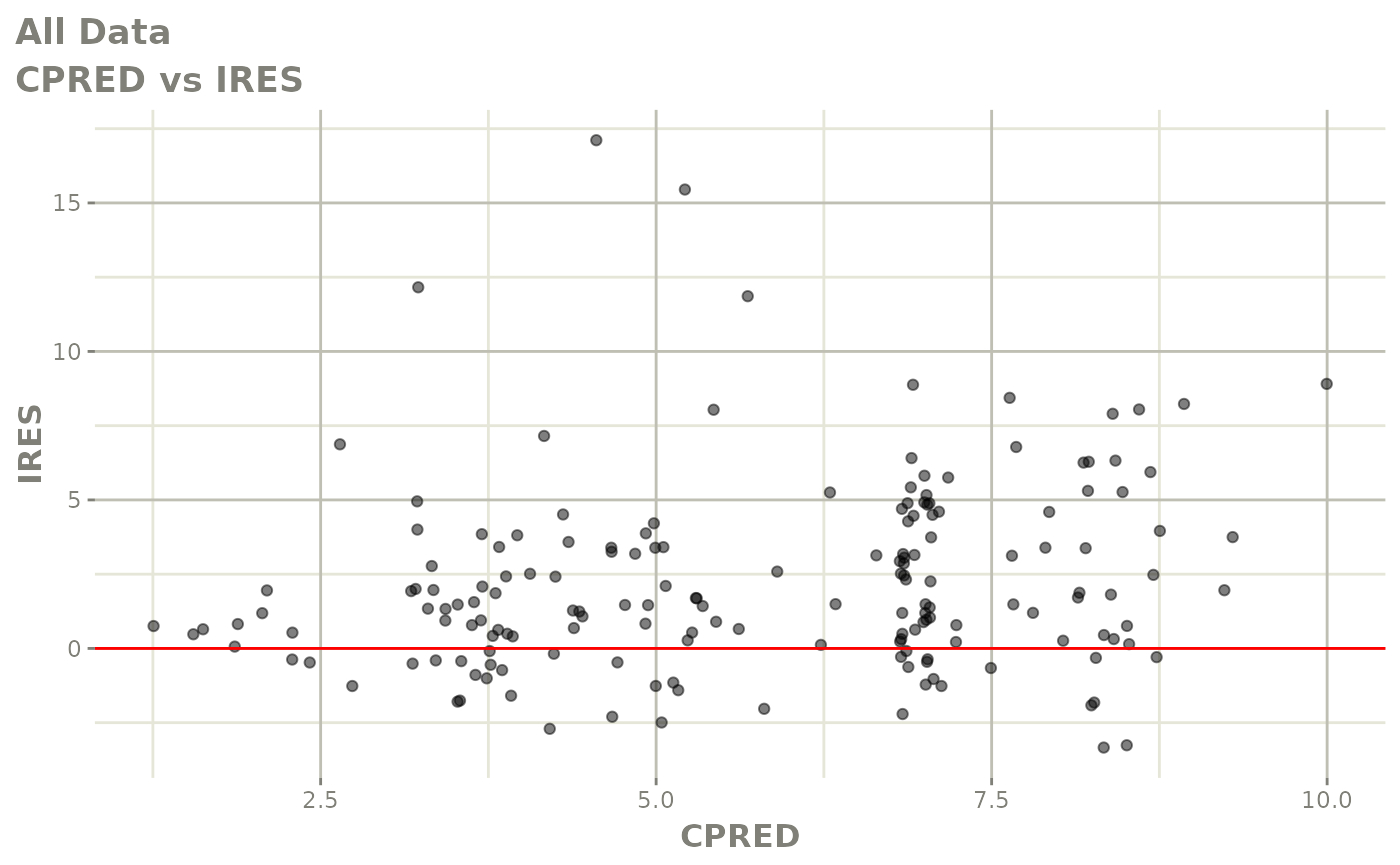
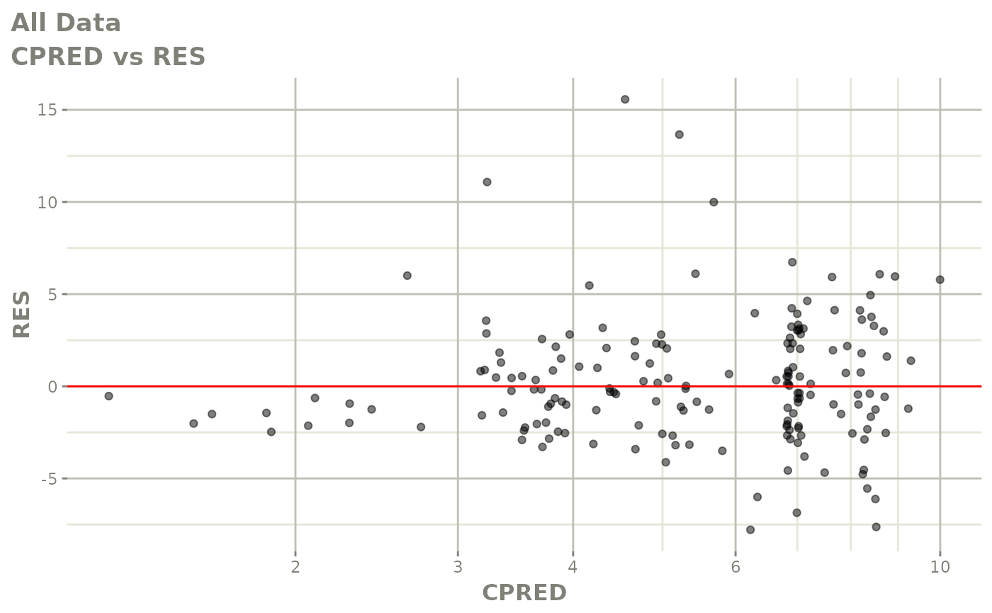
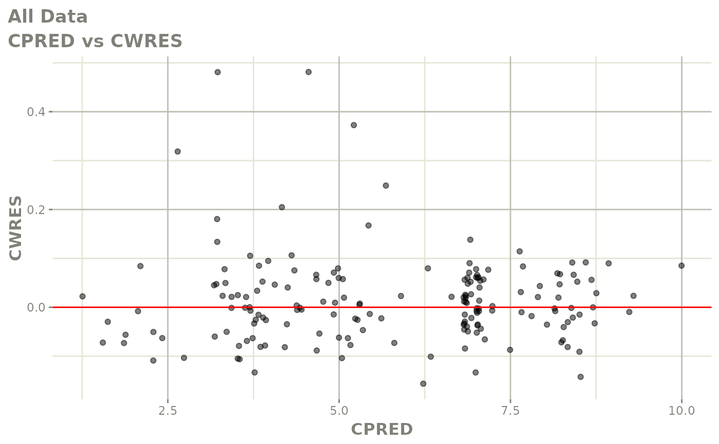
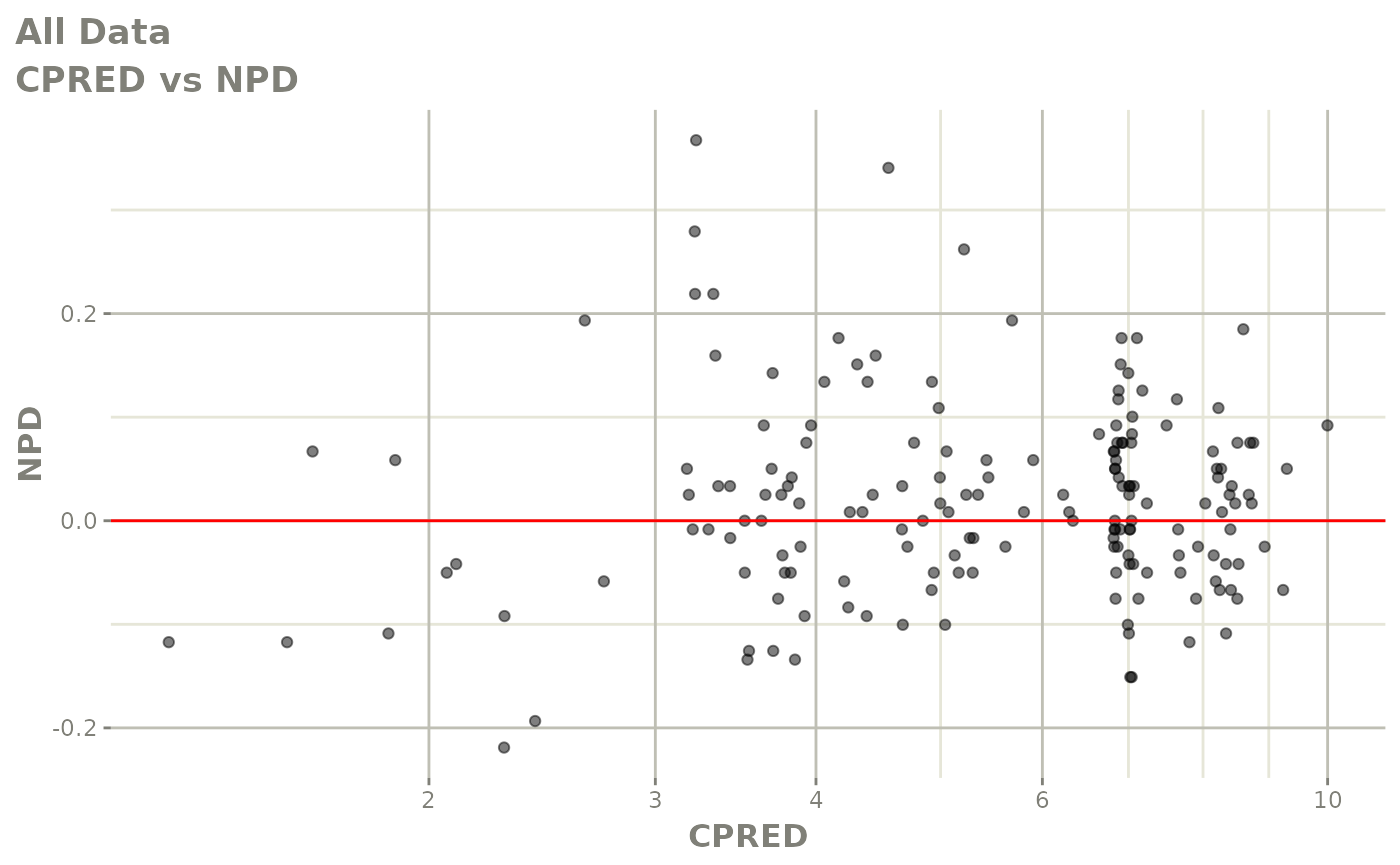
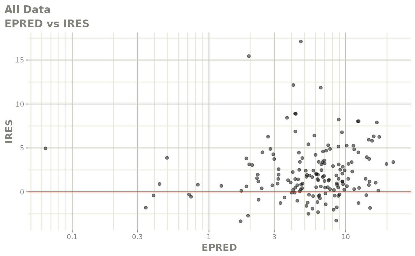
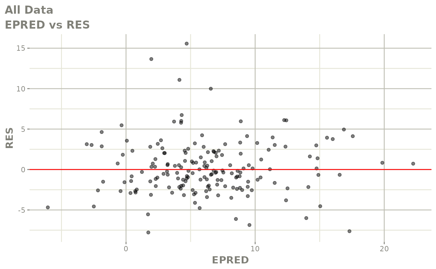
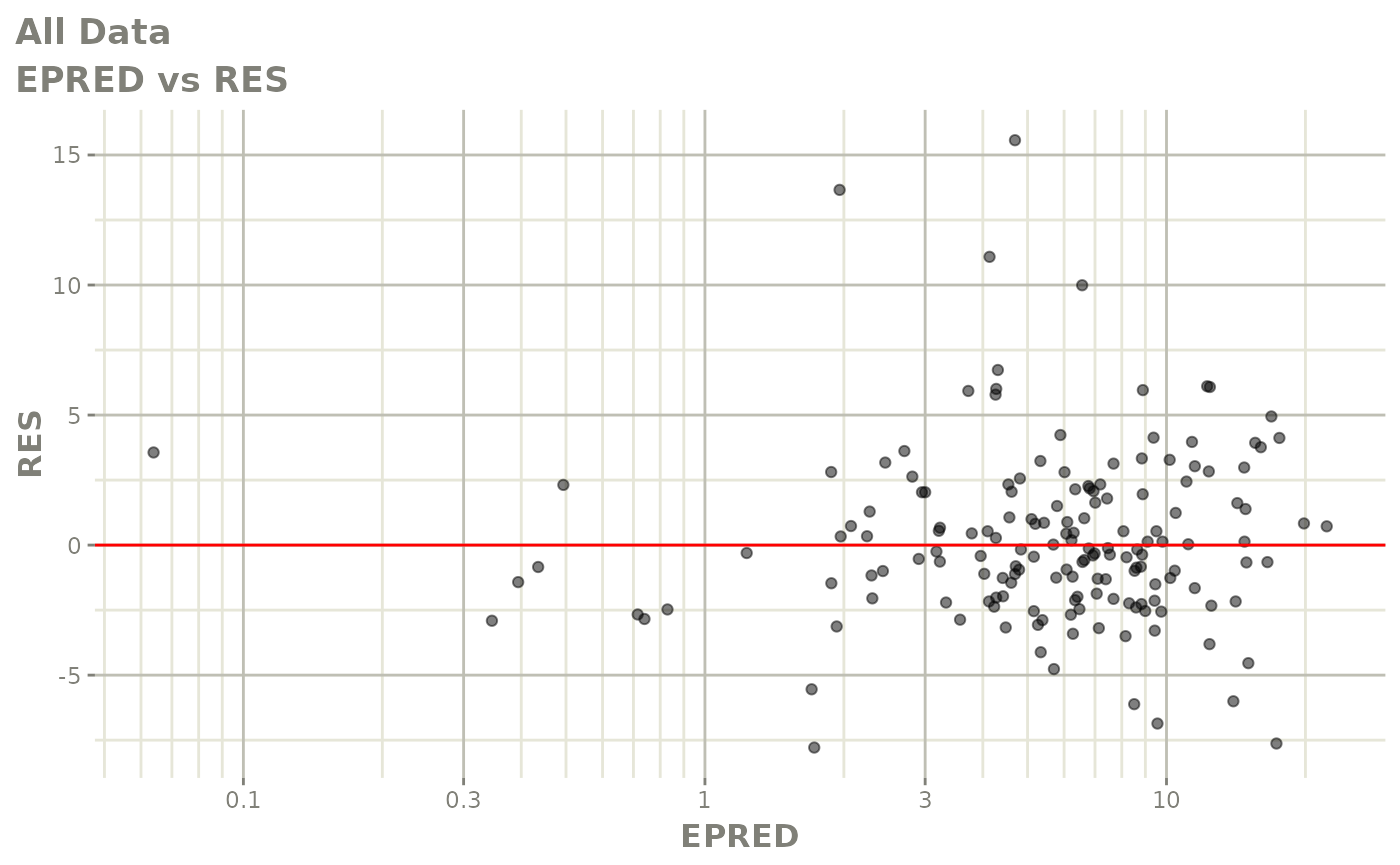
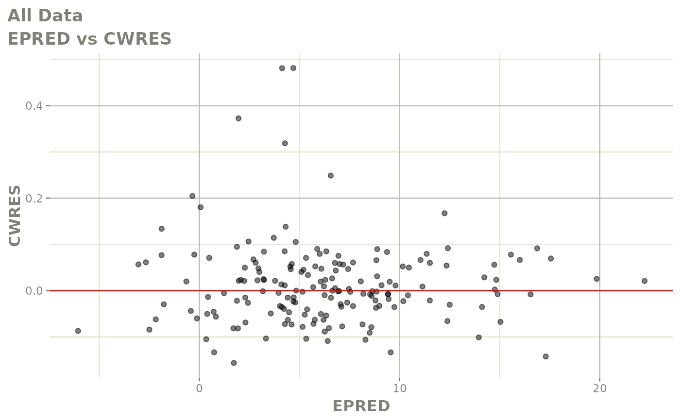
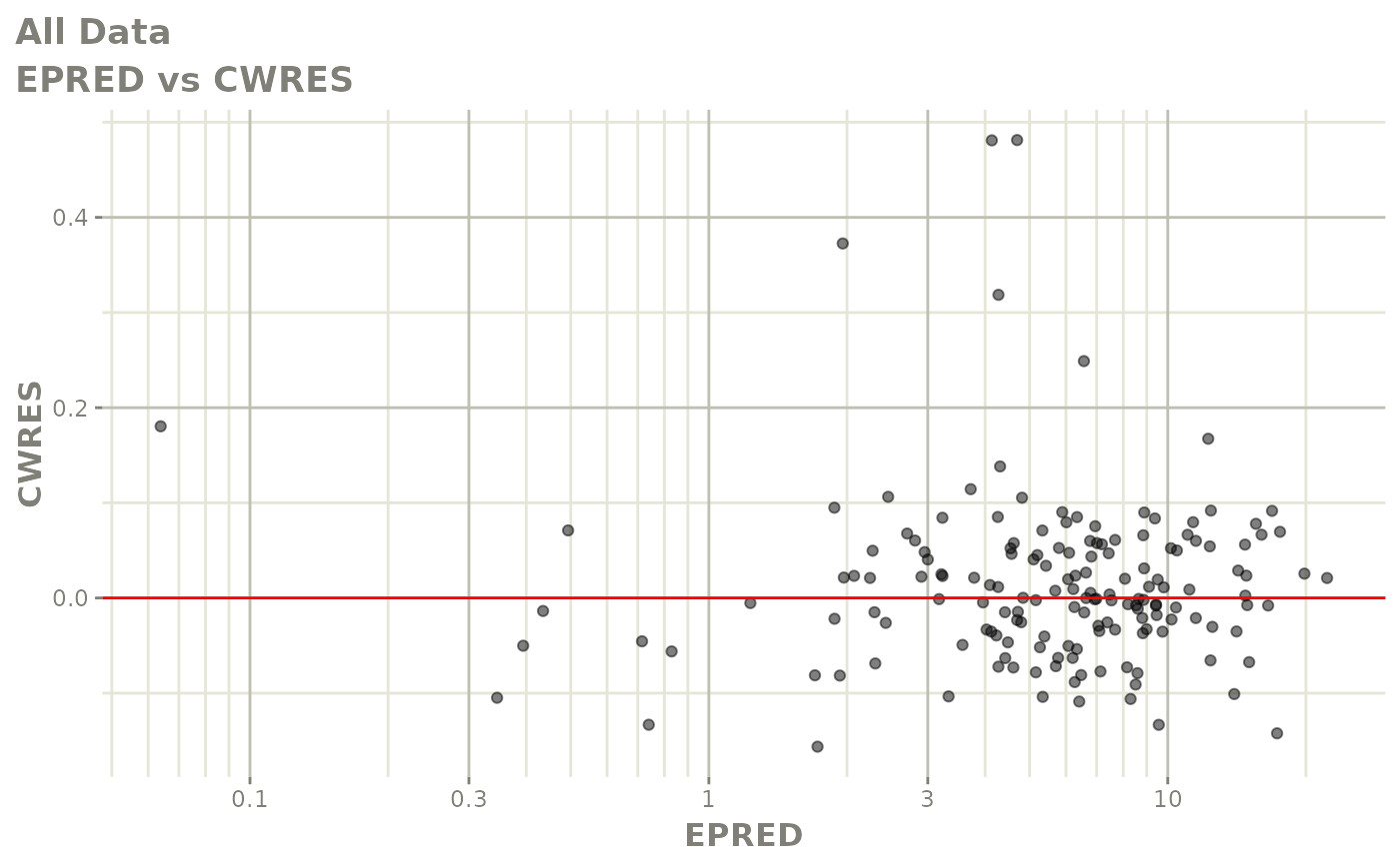
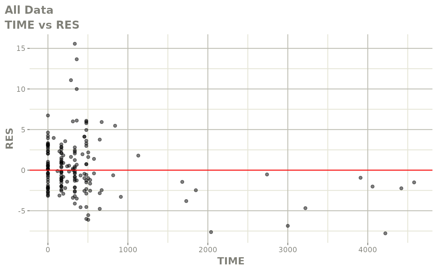
print(res_vs_pred(xpdb) +
      ylab("Conditional Weighted Residuals") +
      xlab("Population Predicted Neutrophil Count (10^9/L)"))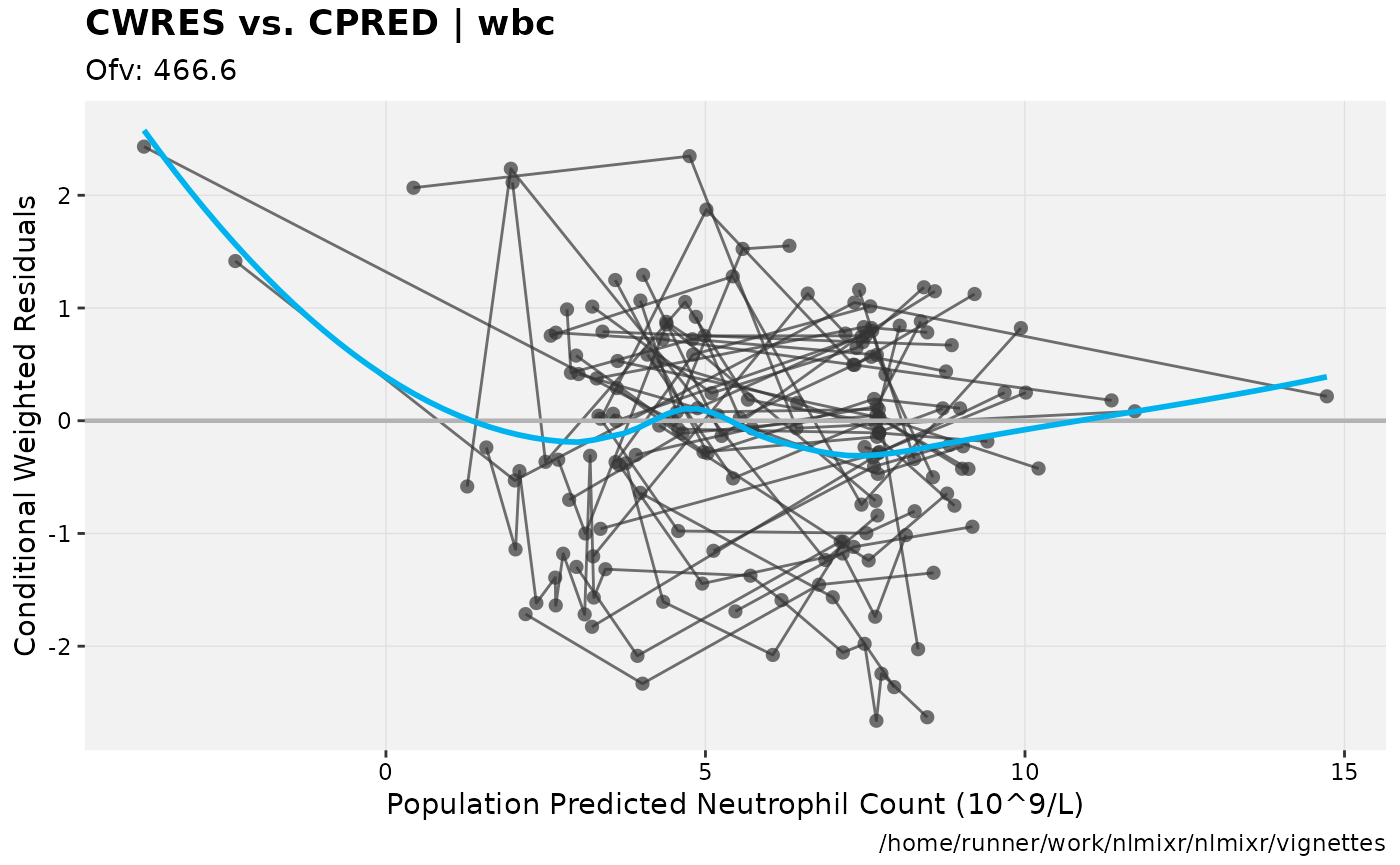


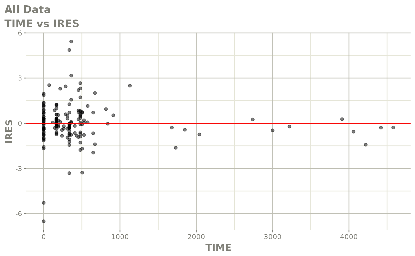
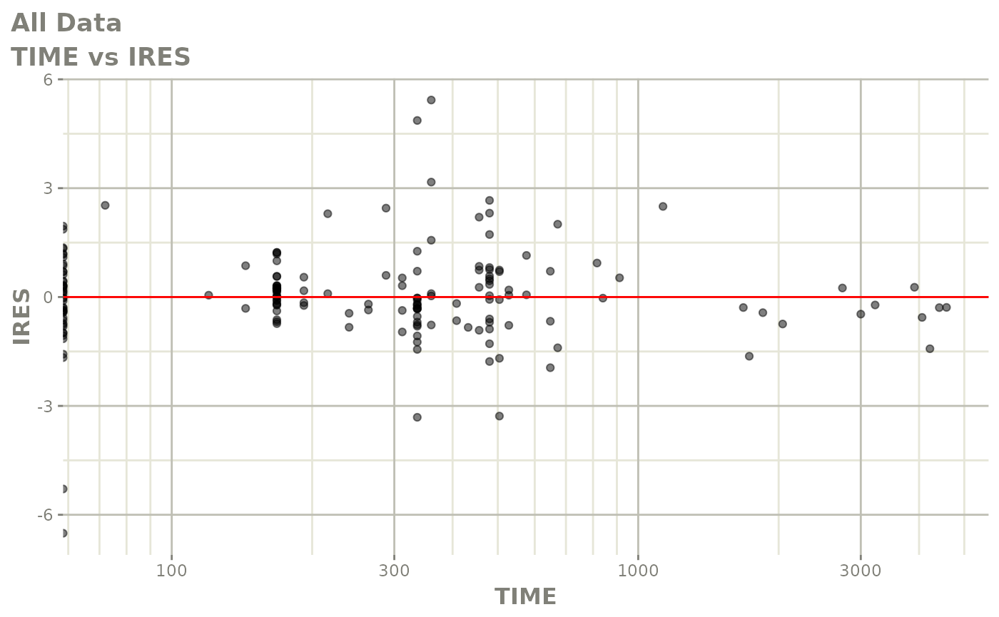
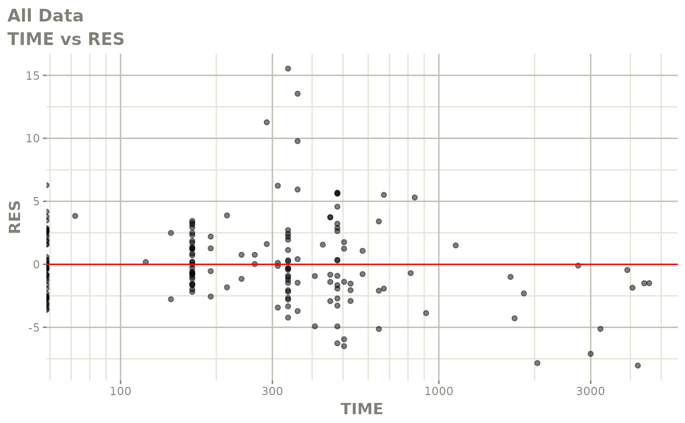
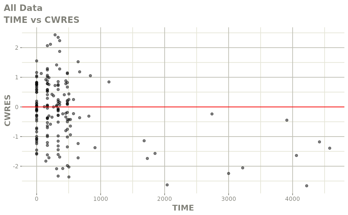
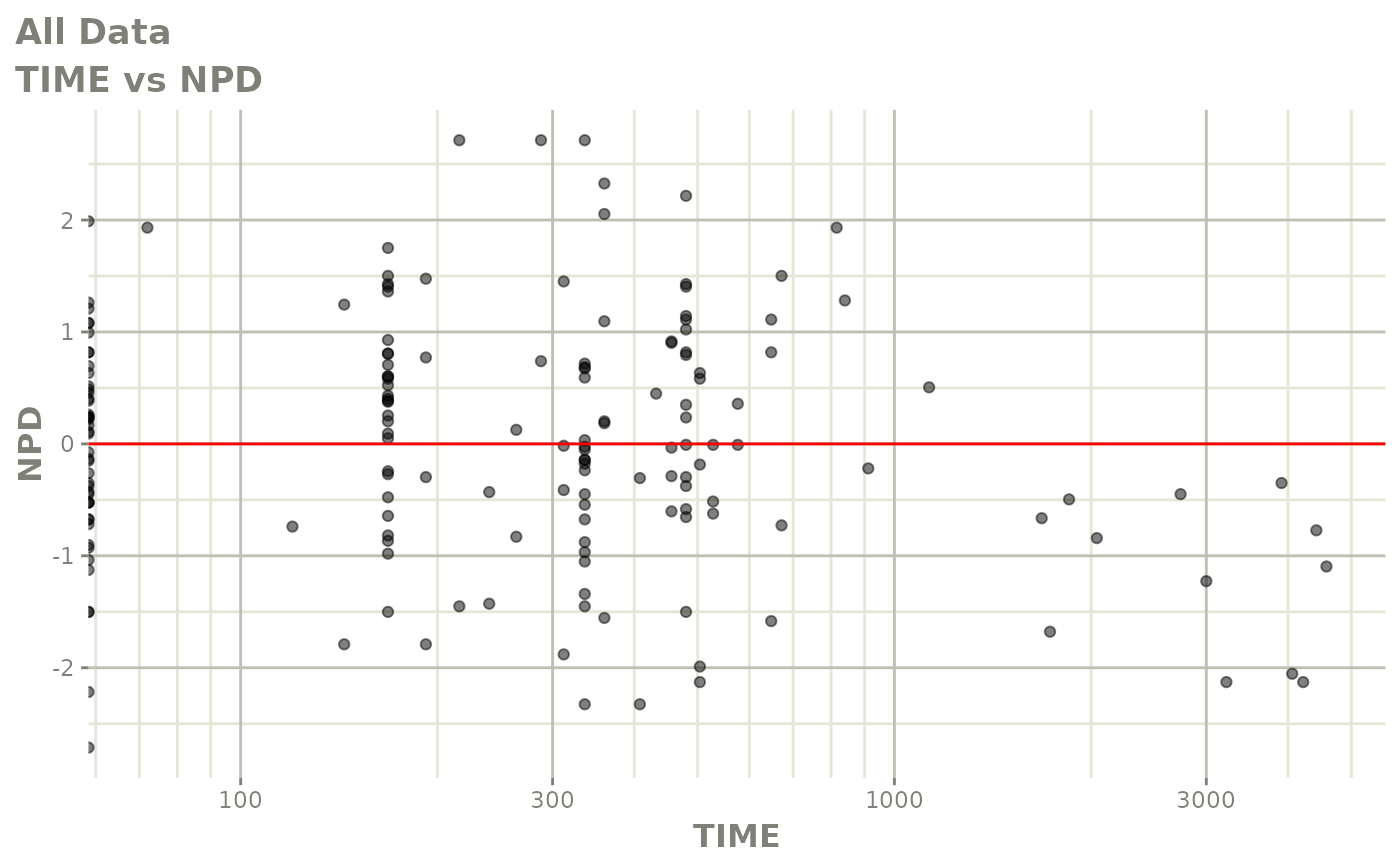
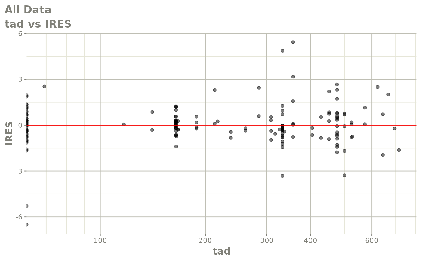
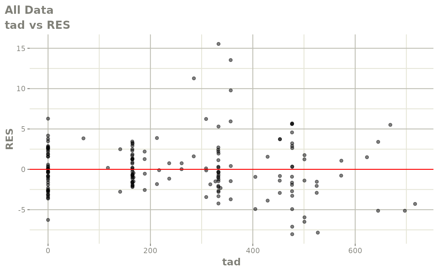
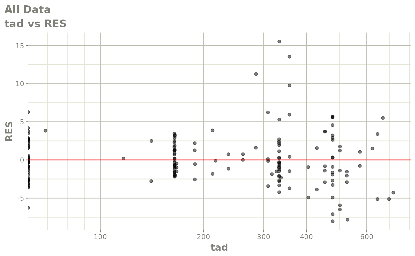
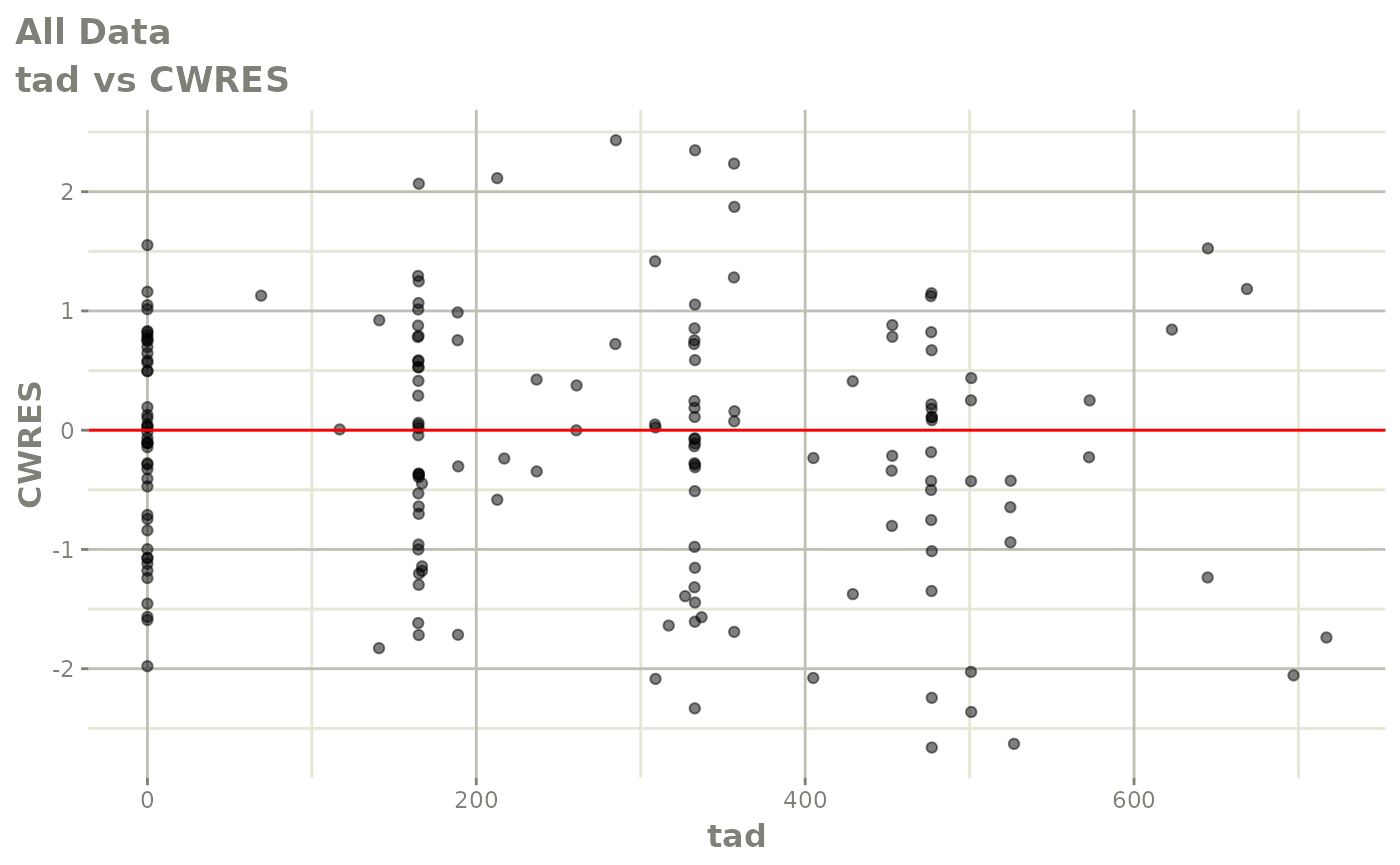
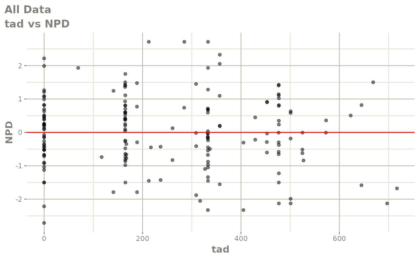
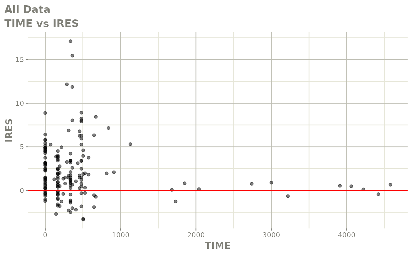
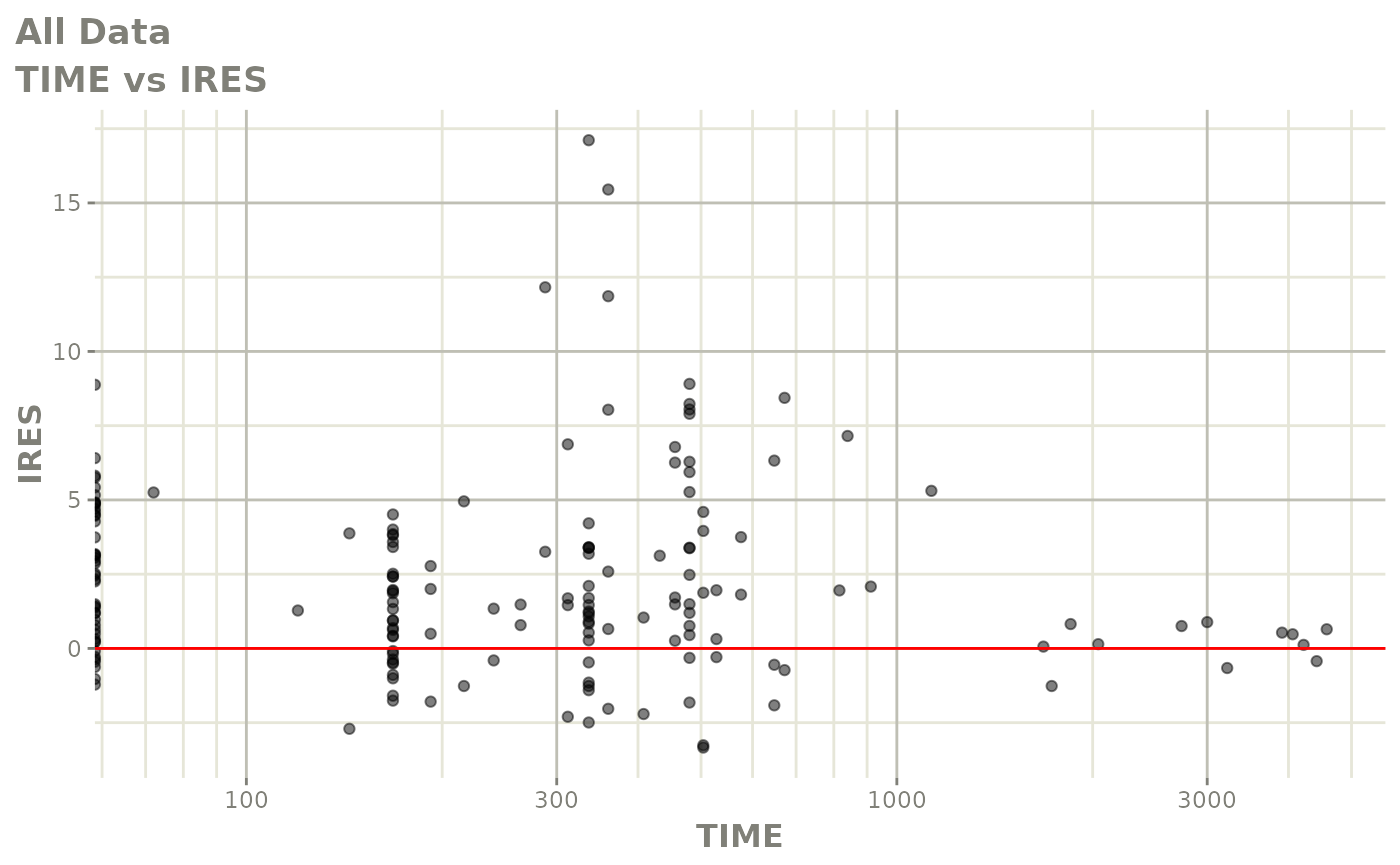
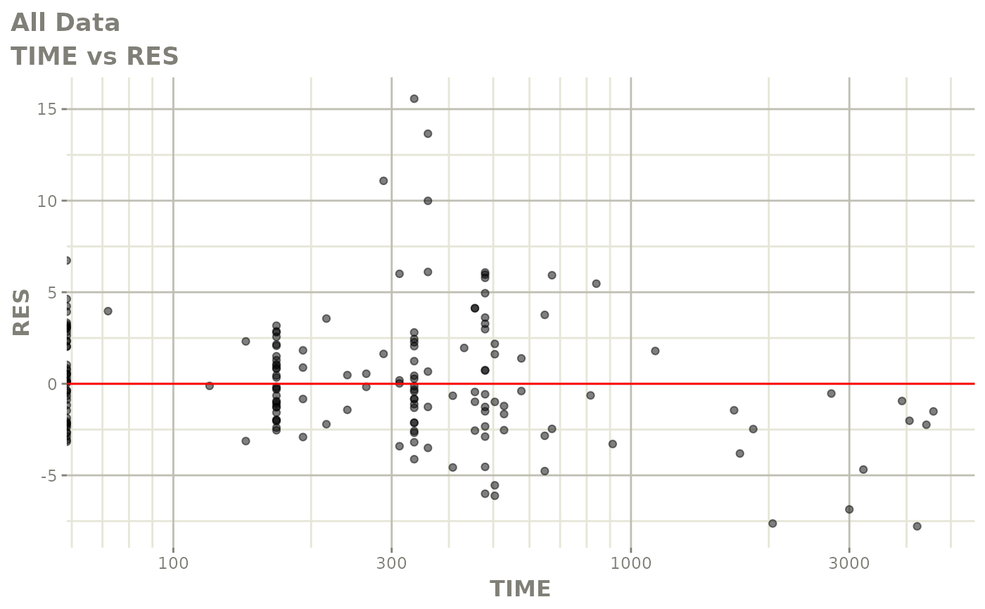
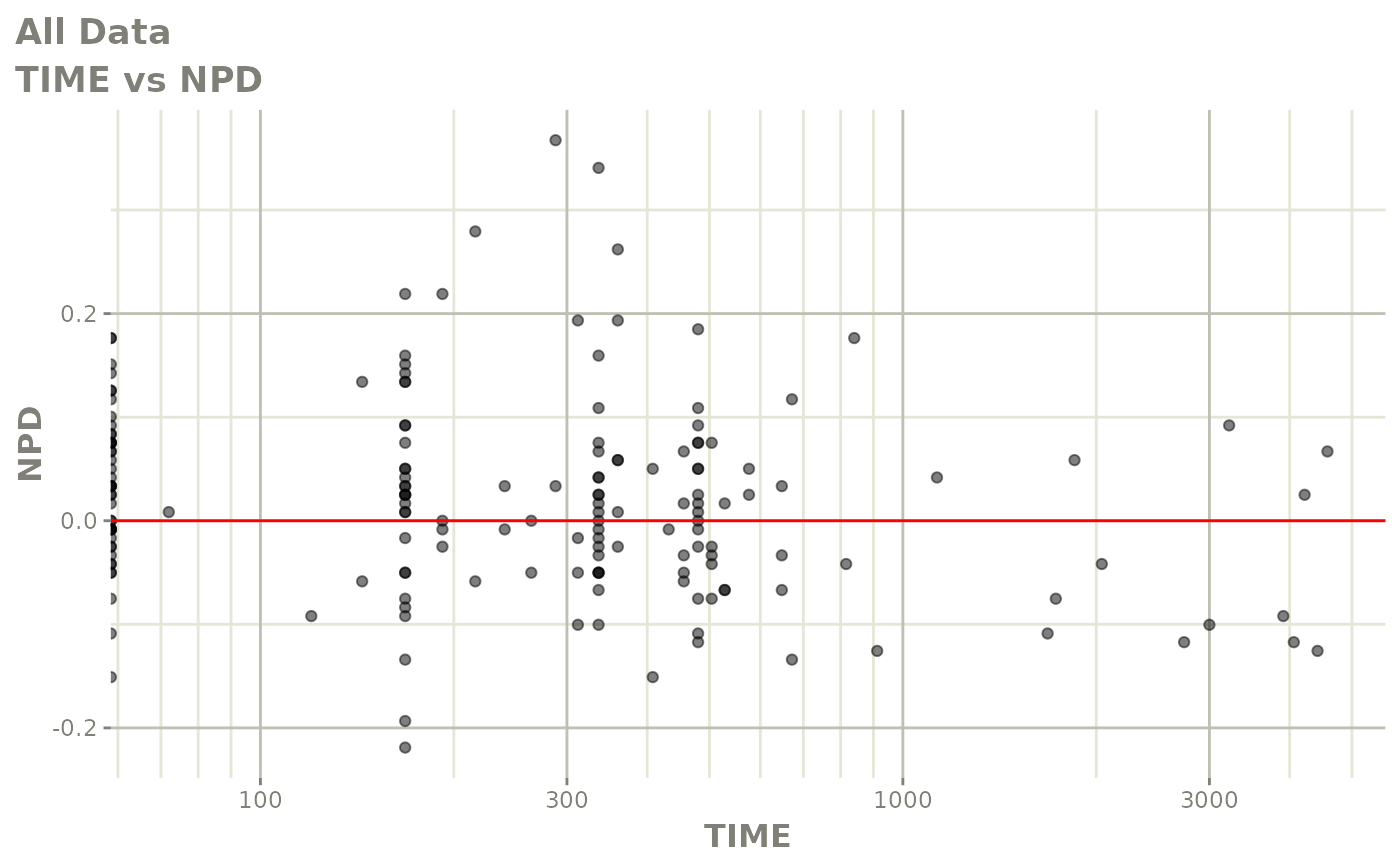
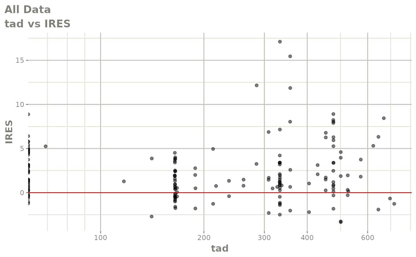
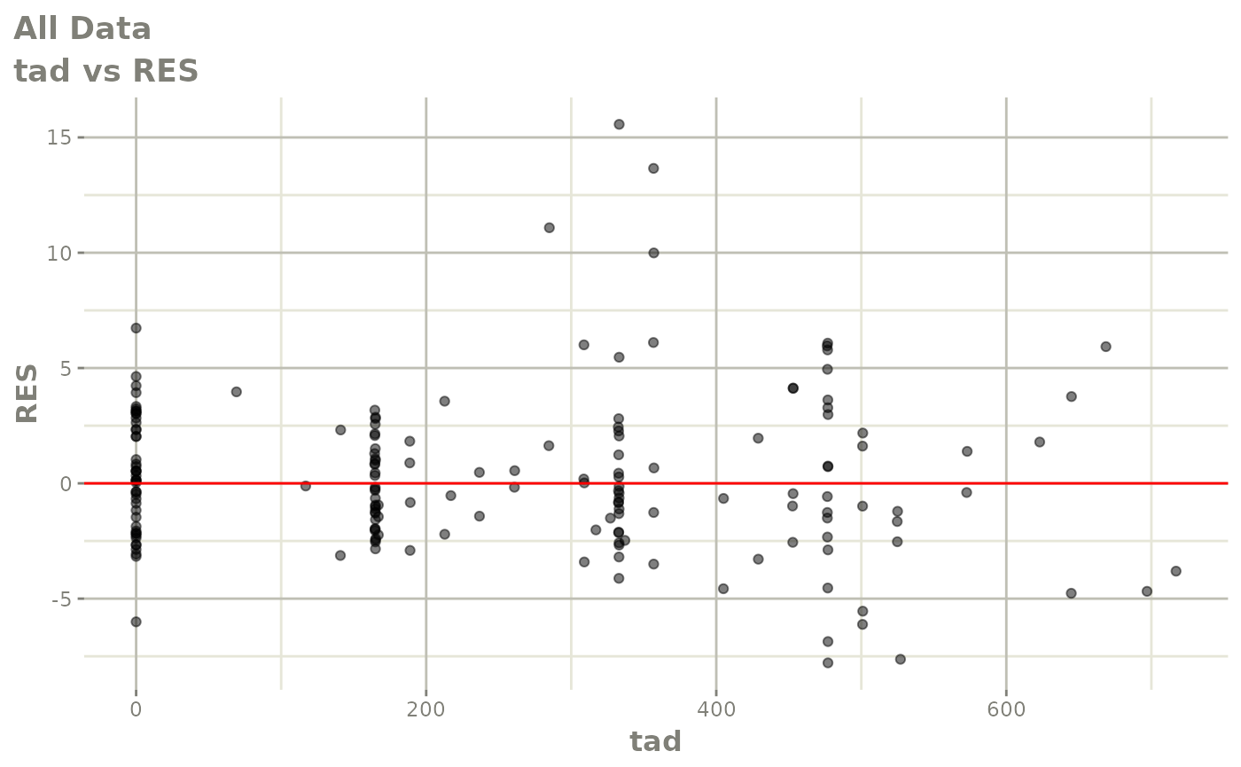
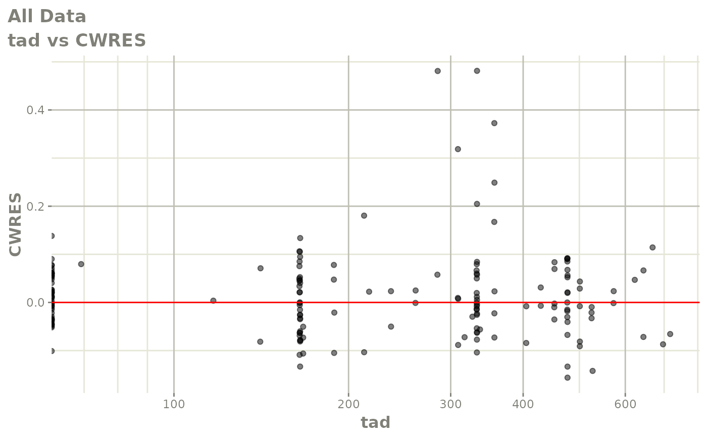
print(res_vs_idv(xpdb) +
      ylab("Conditional Weighted Residuals") +
      xlab("Time (h)"))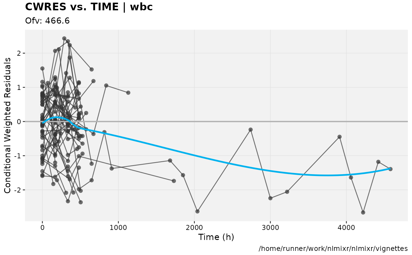


print(prm_vs_iteration(xpdb))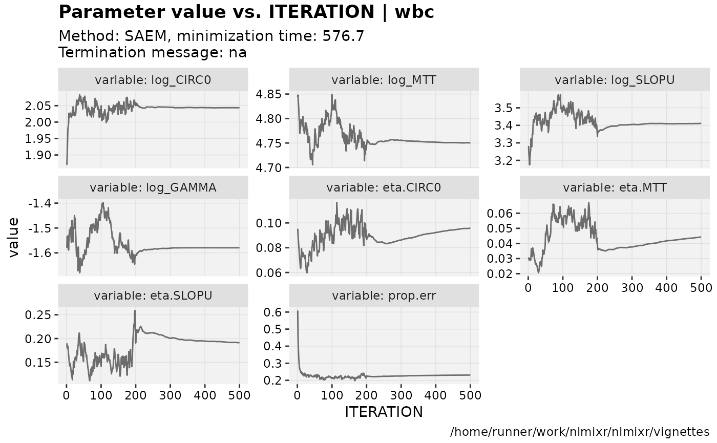


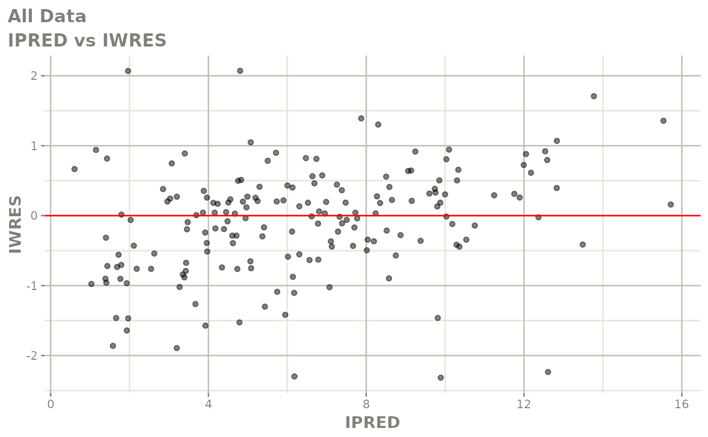
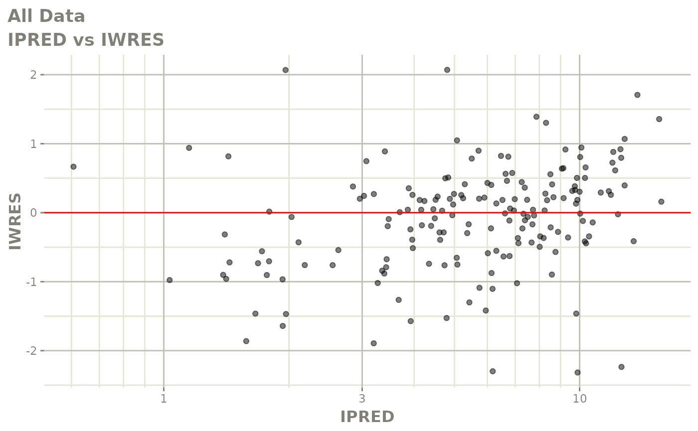
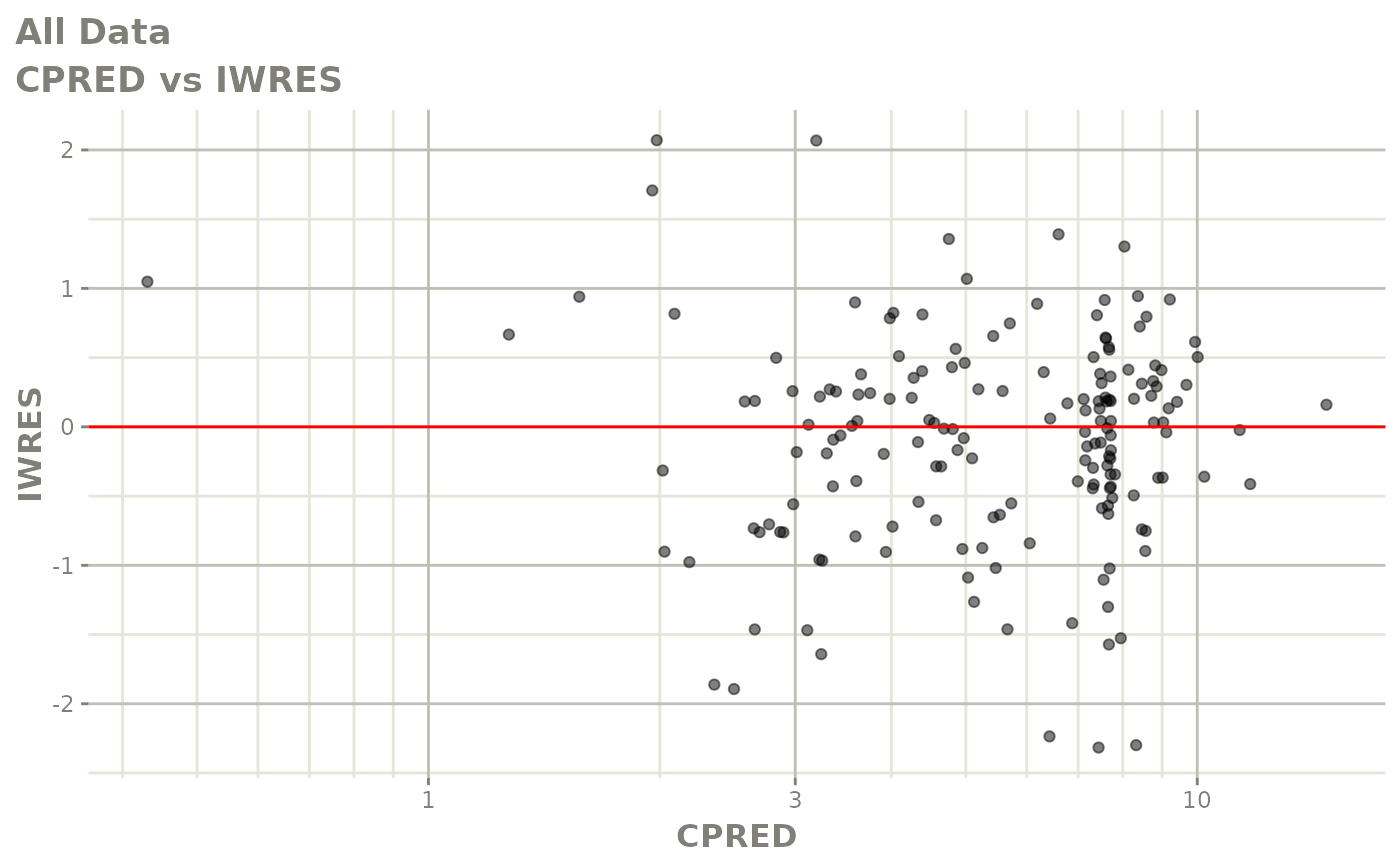
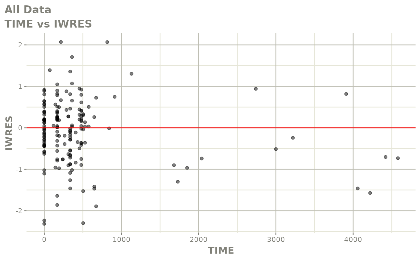
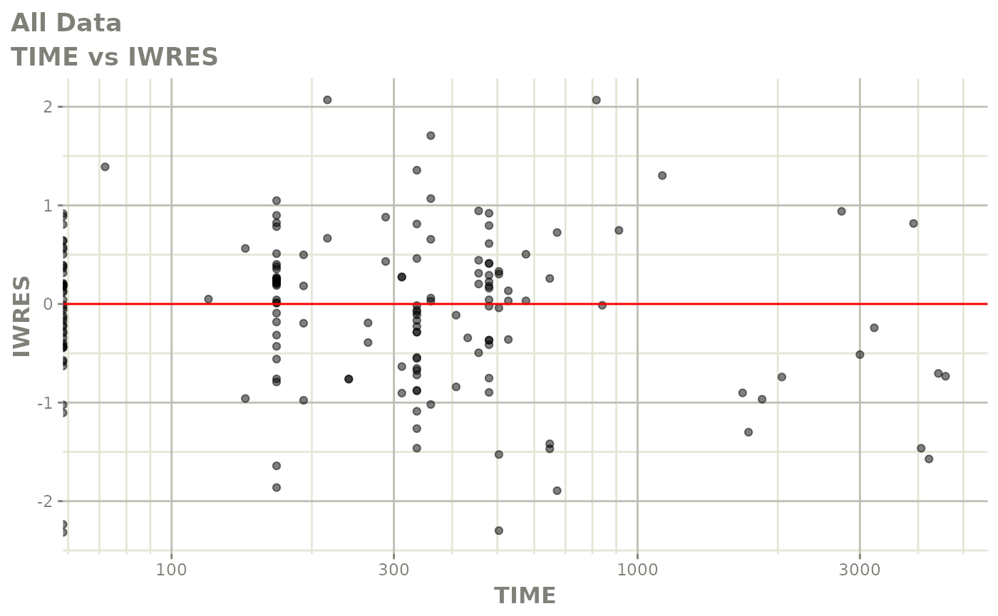
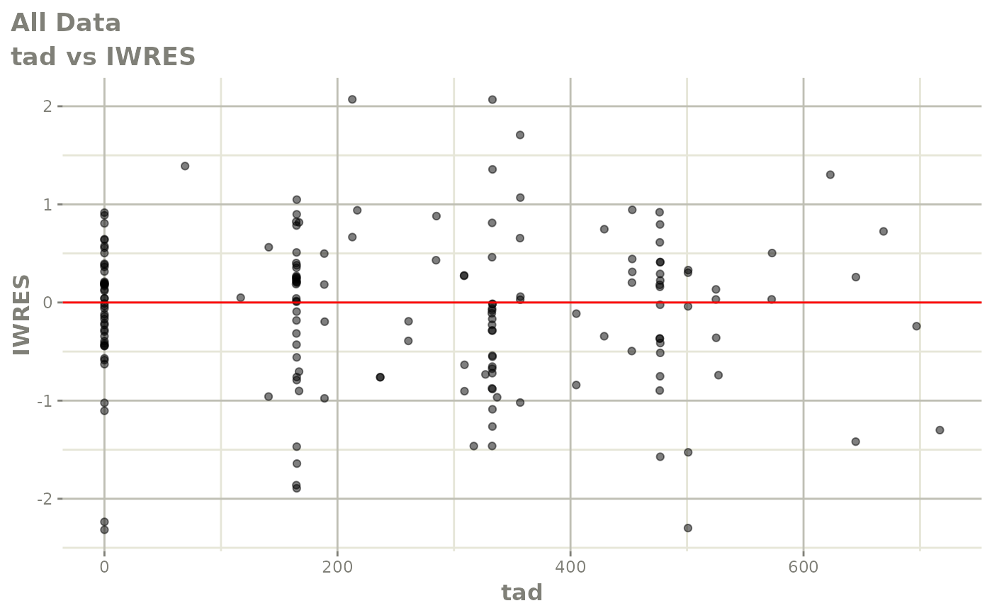
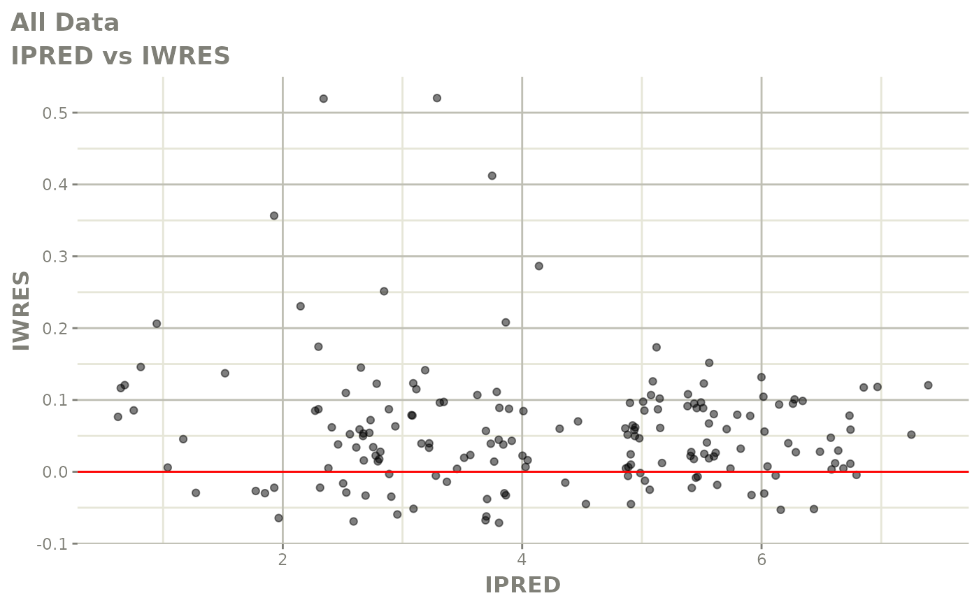
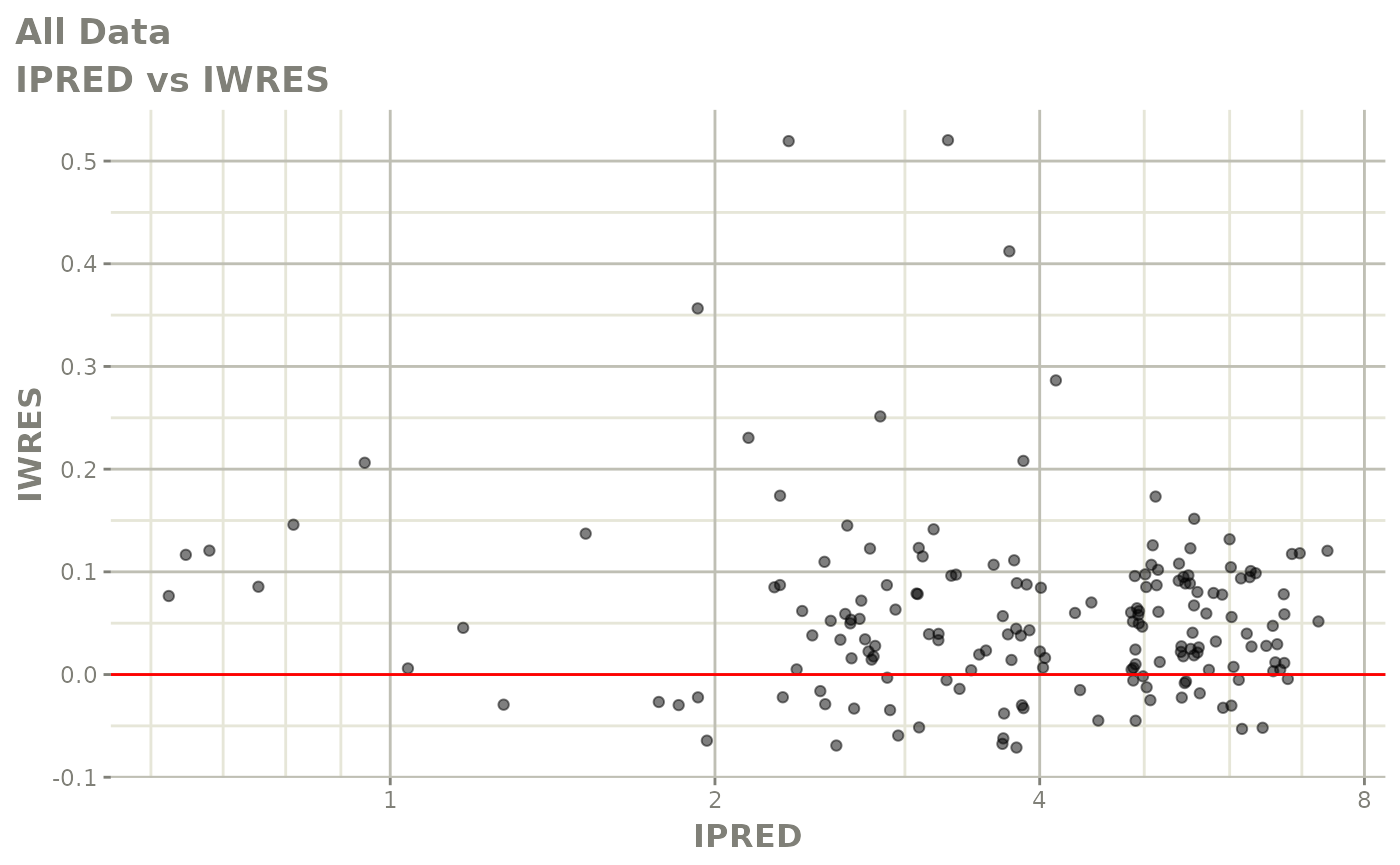
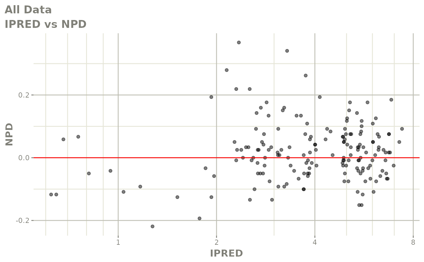
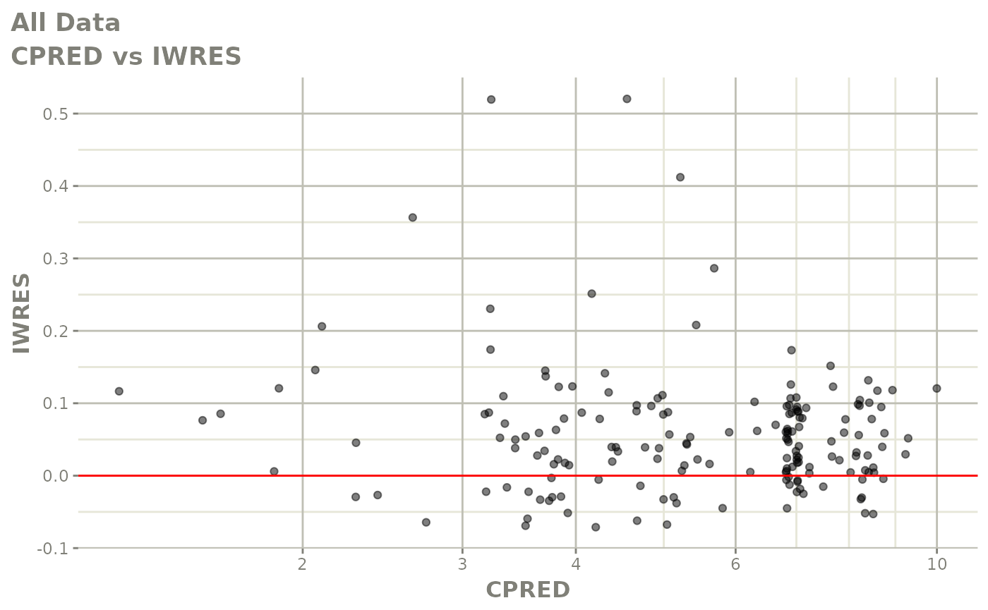
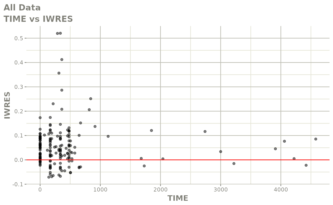
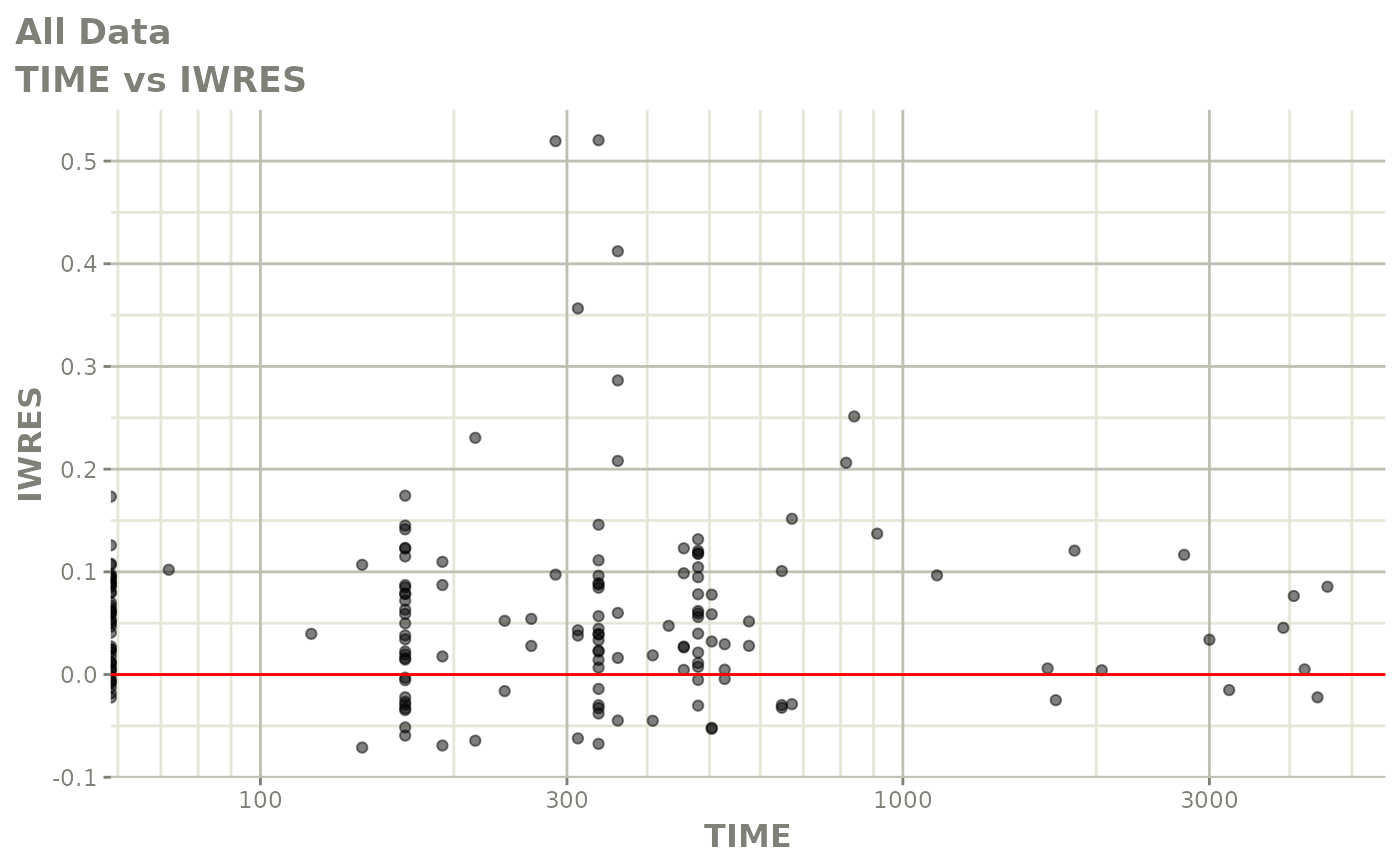
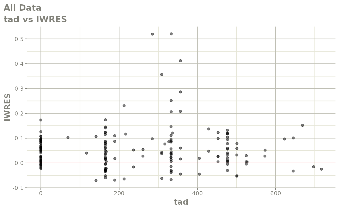
print(absval_res_vs_idv(xpdb, res = 'IWRES') +
      ylab("Individual Weighted Residuals") +
      xlab("Time (h)"))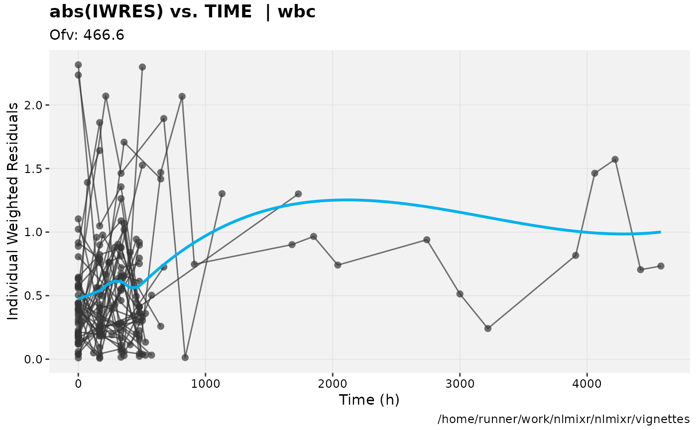


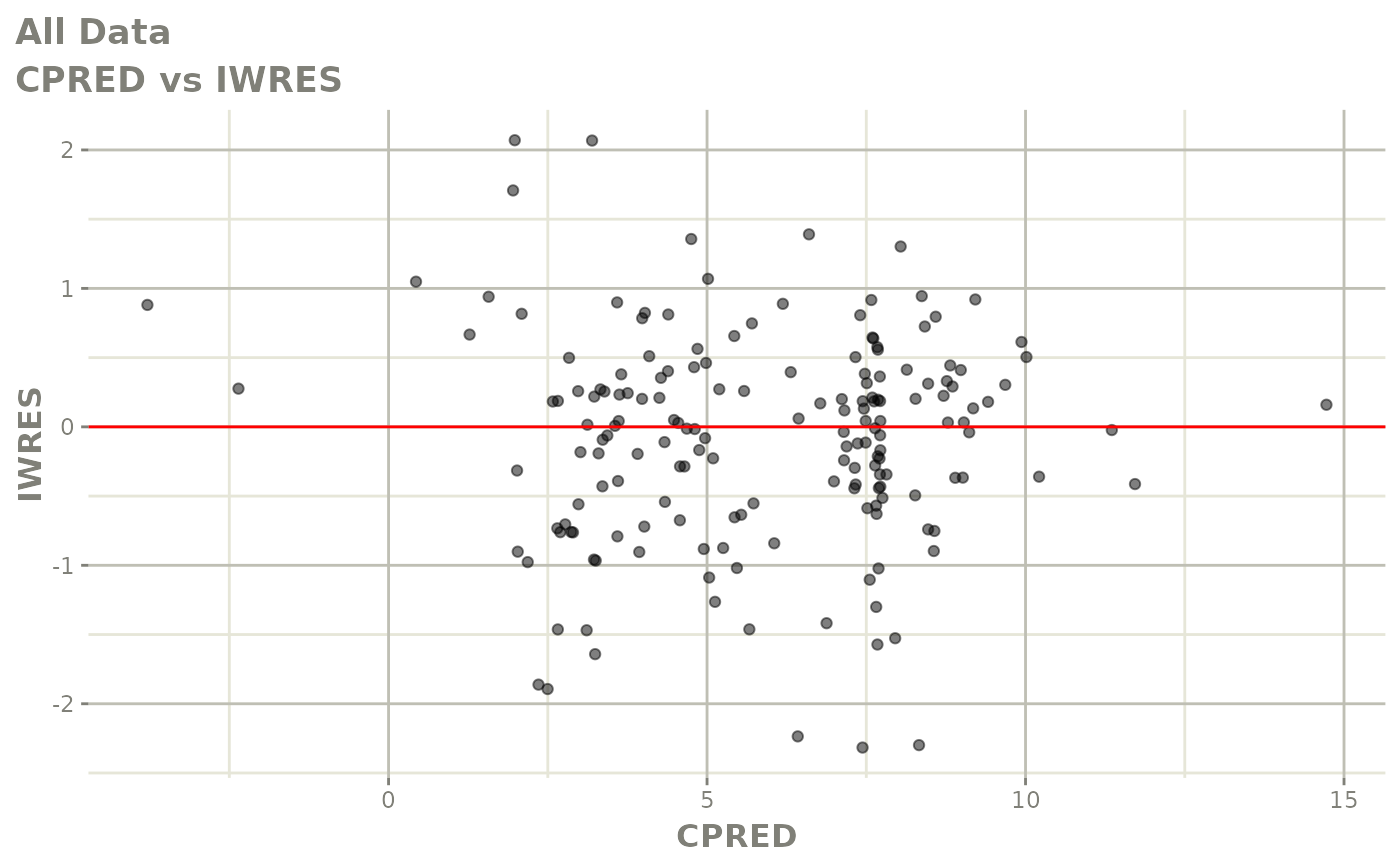
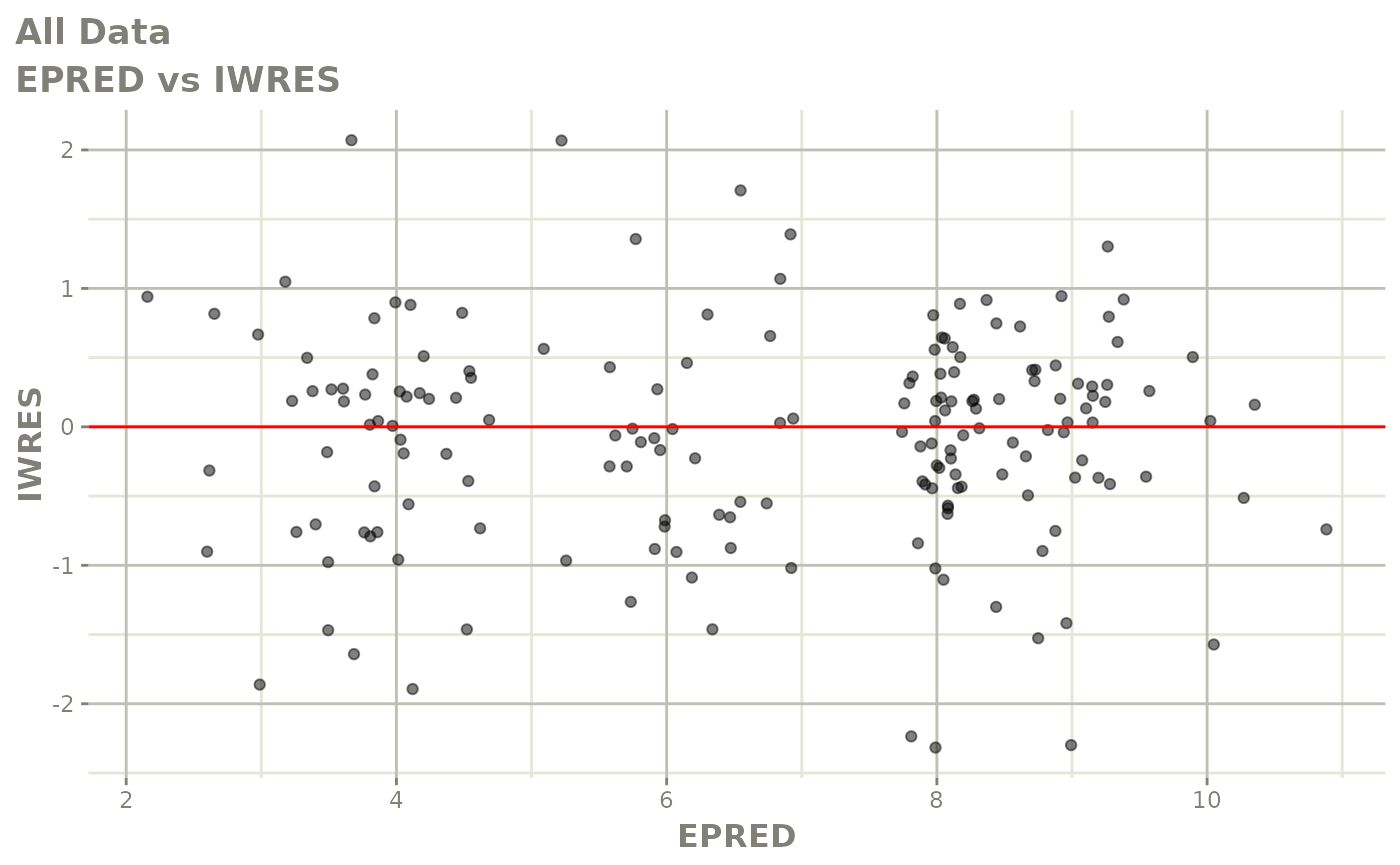
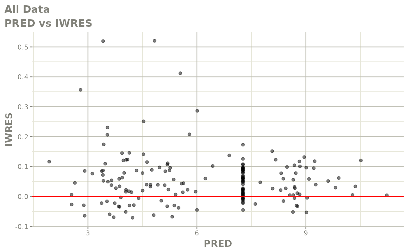
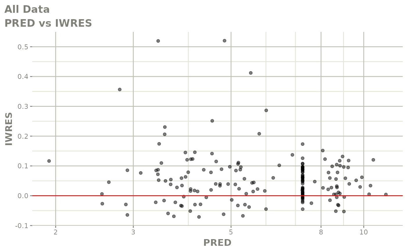
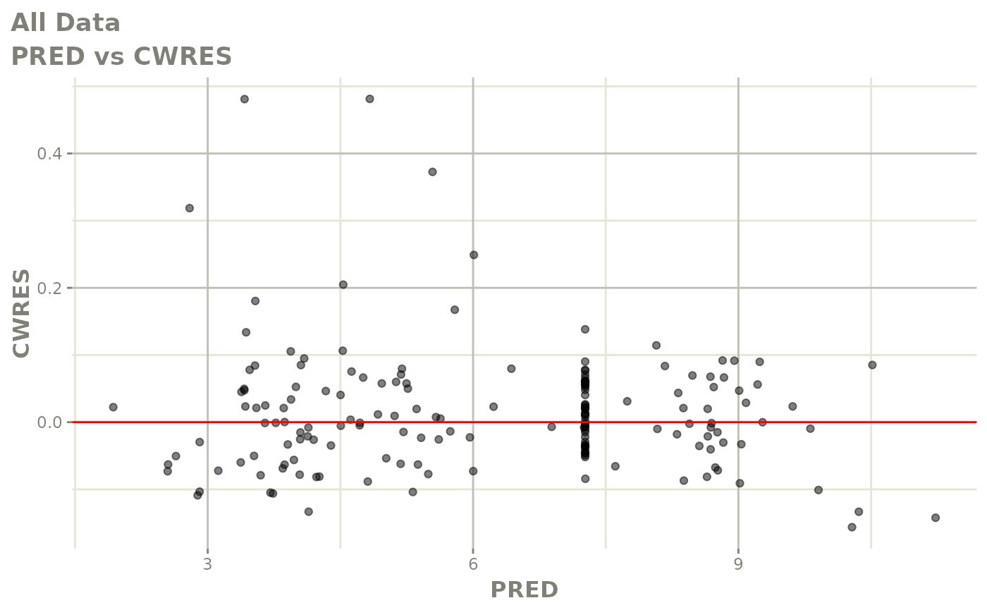
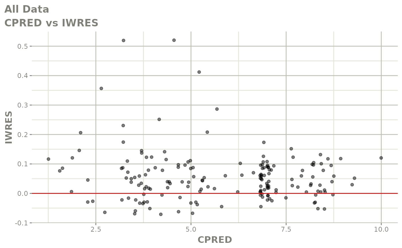
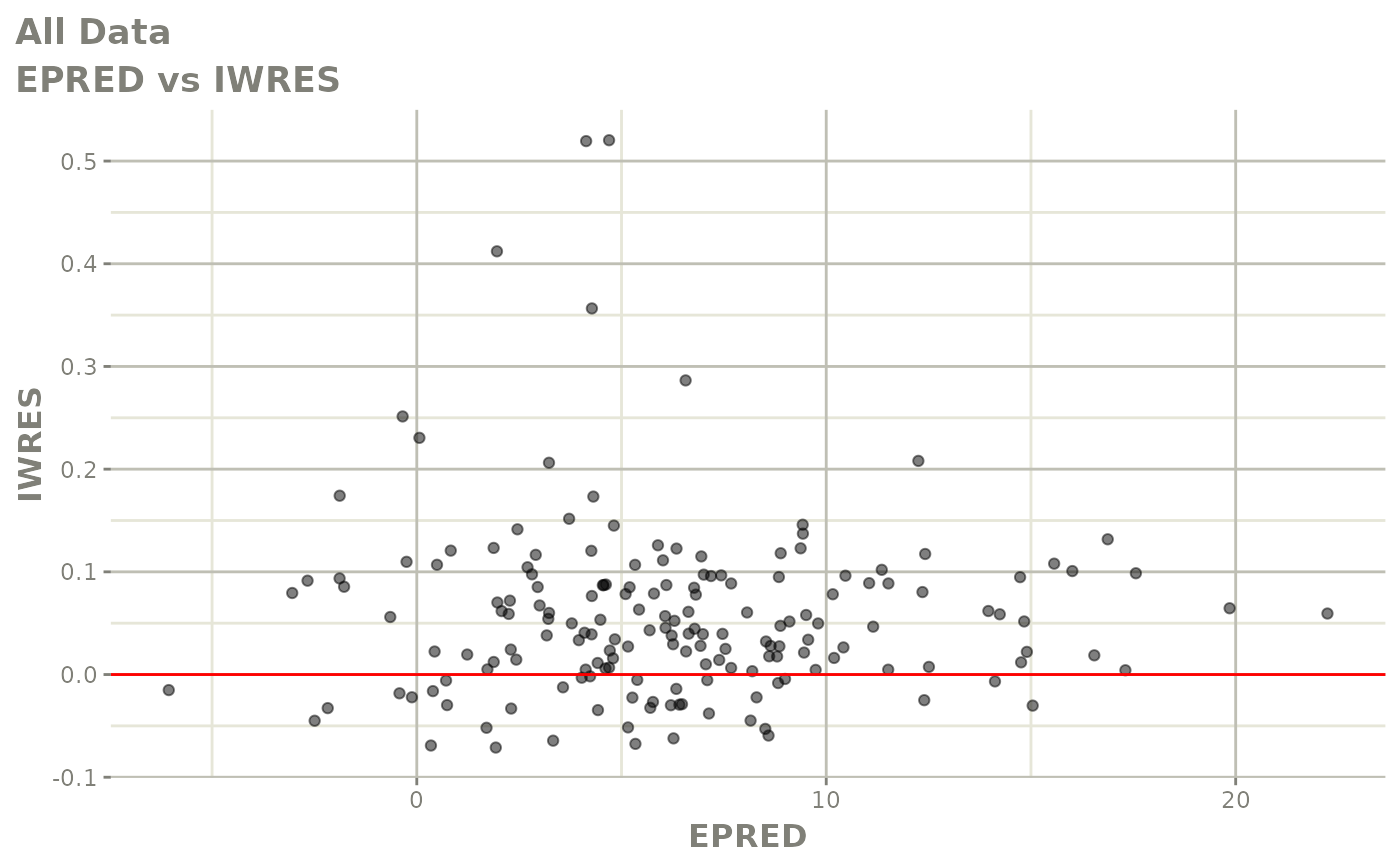
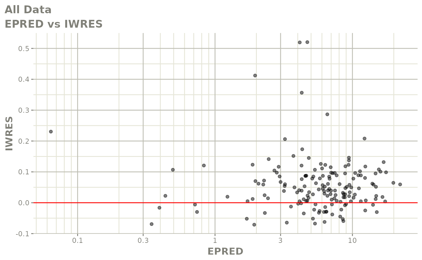
print(absval_res_vs_pred(xpdb, res = 'IWRES') +
      ylab("Individual Weighted Residuals") +
      xlab("Population Predicted Neutrophil Count (10^9/L)"))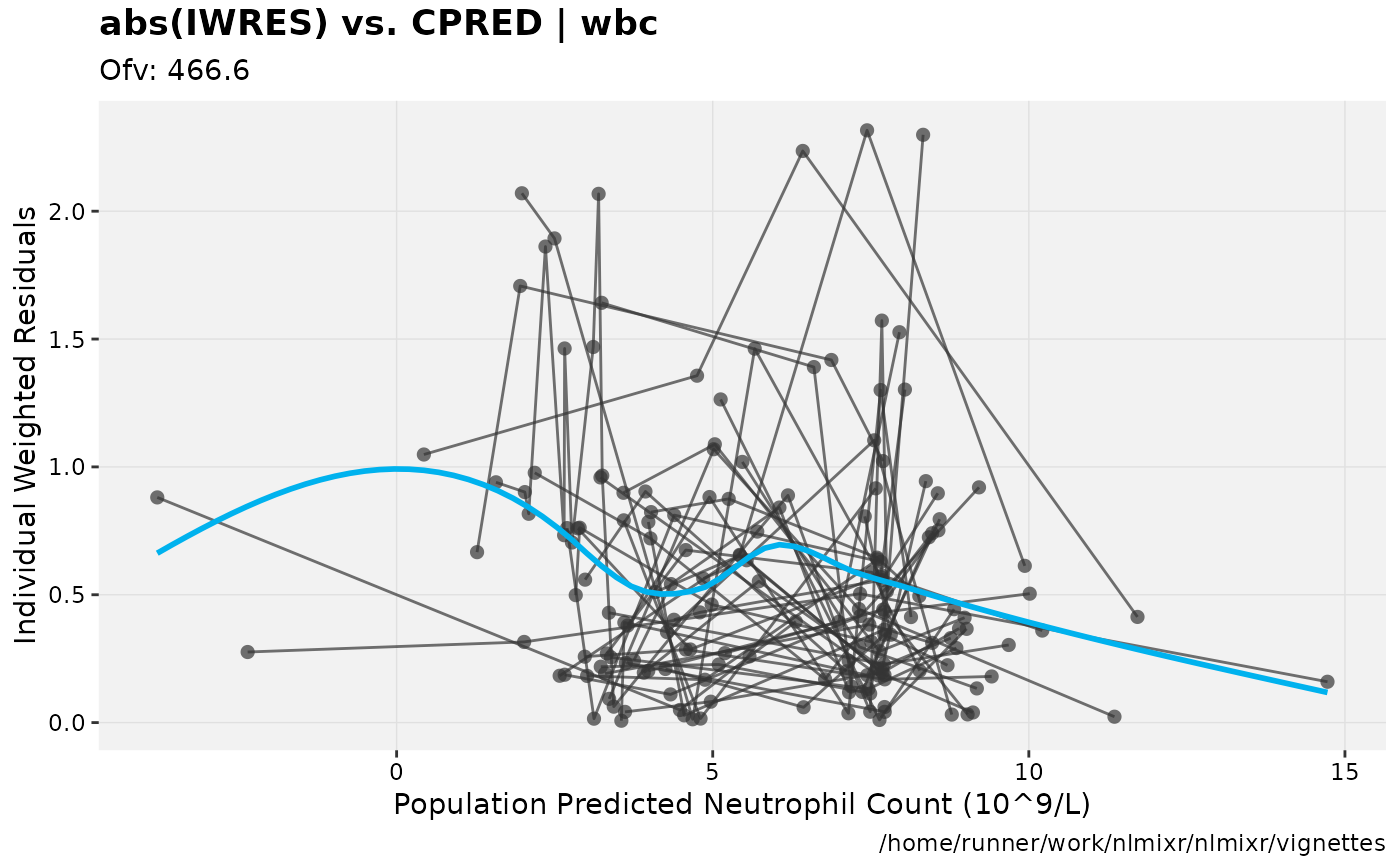


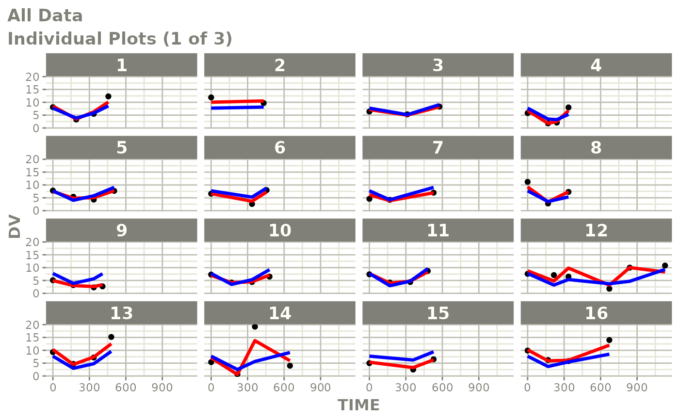
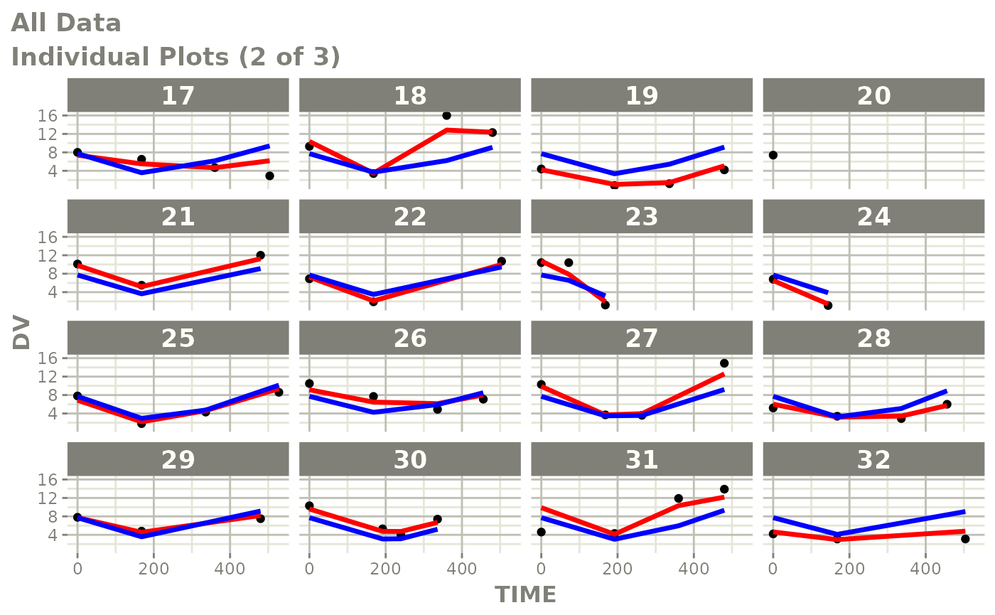
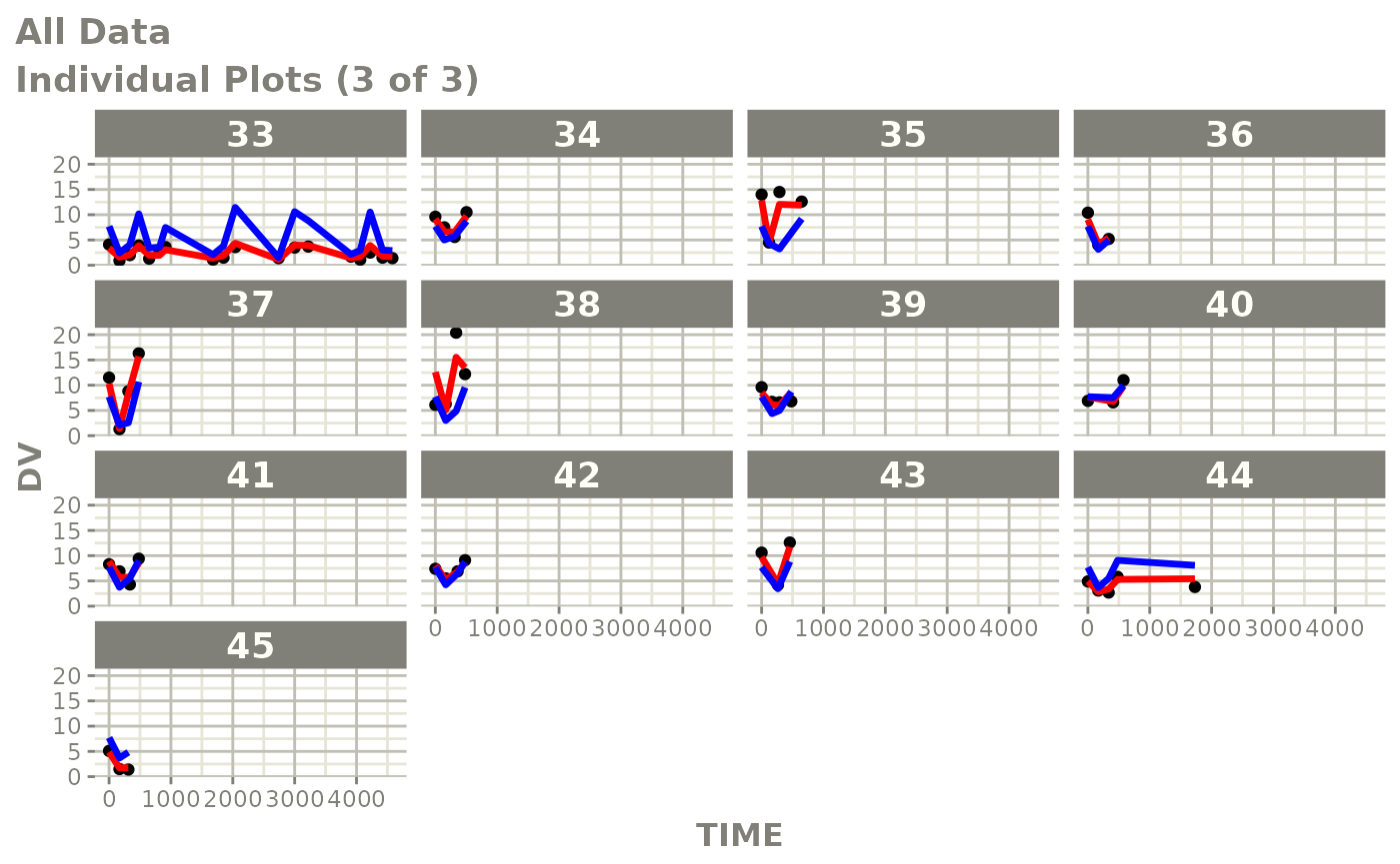
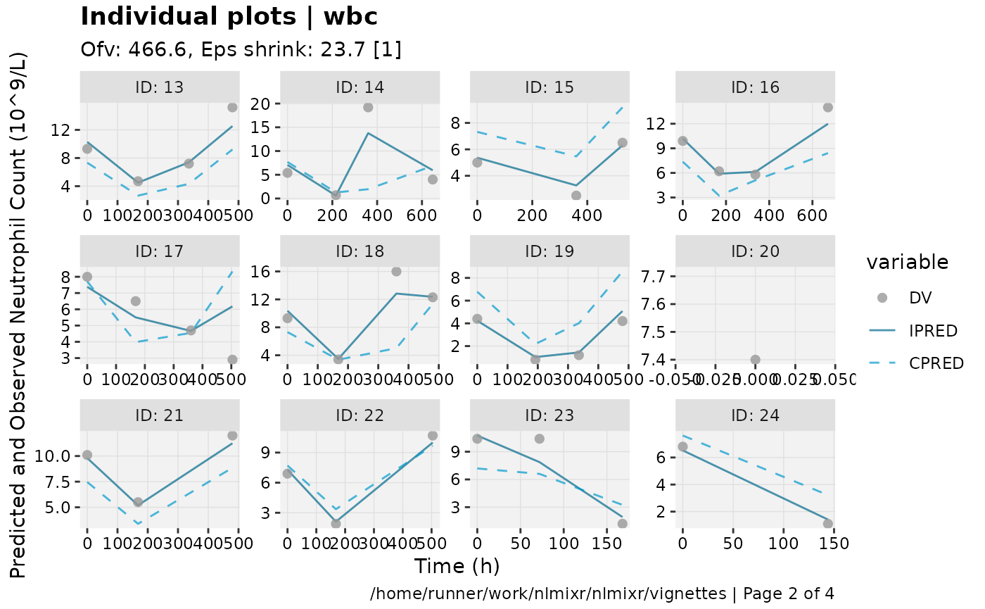
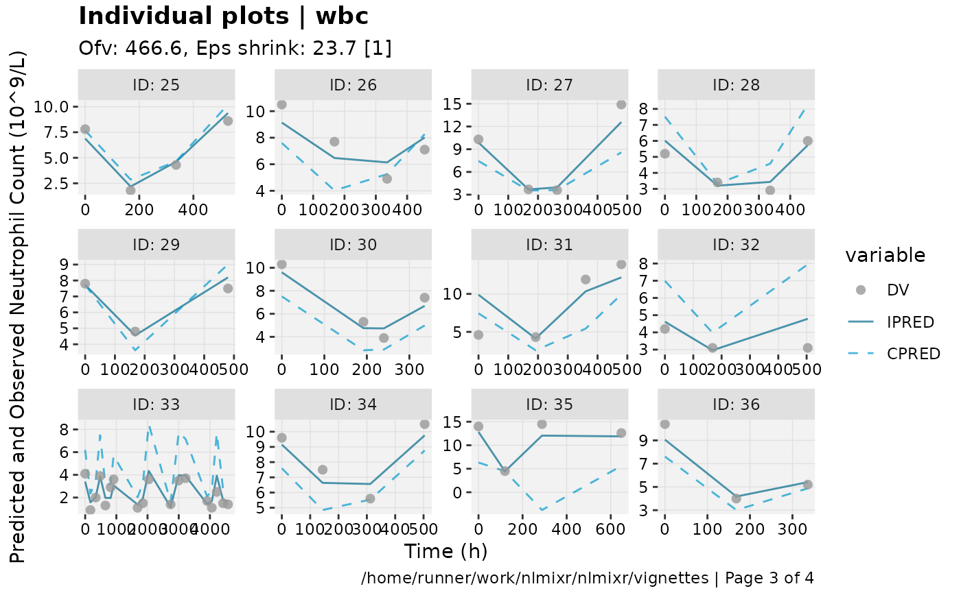
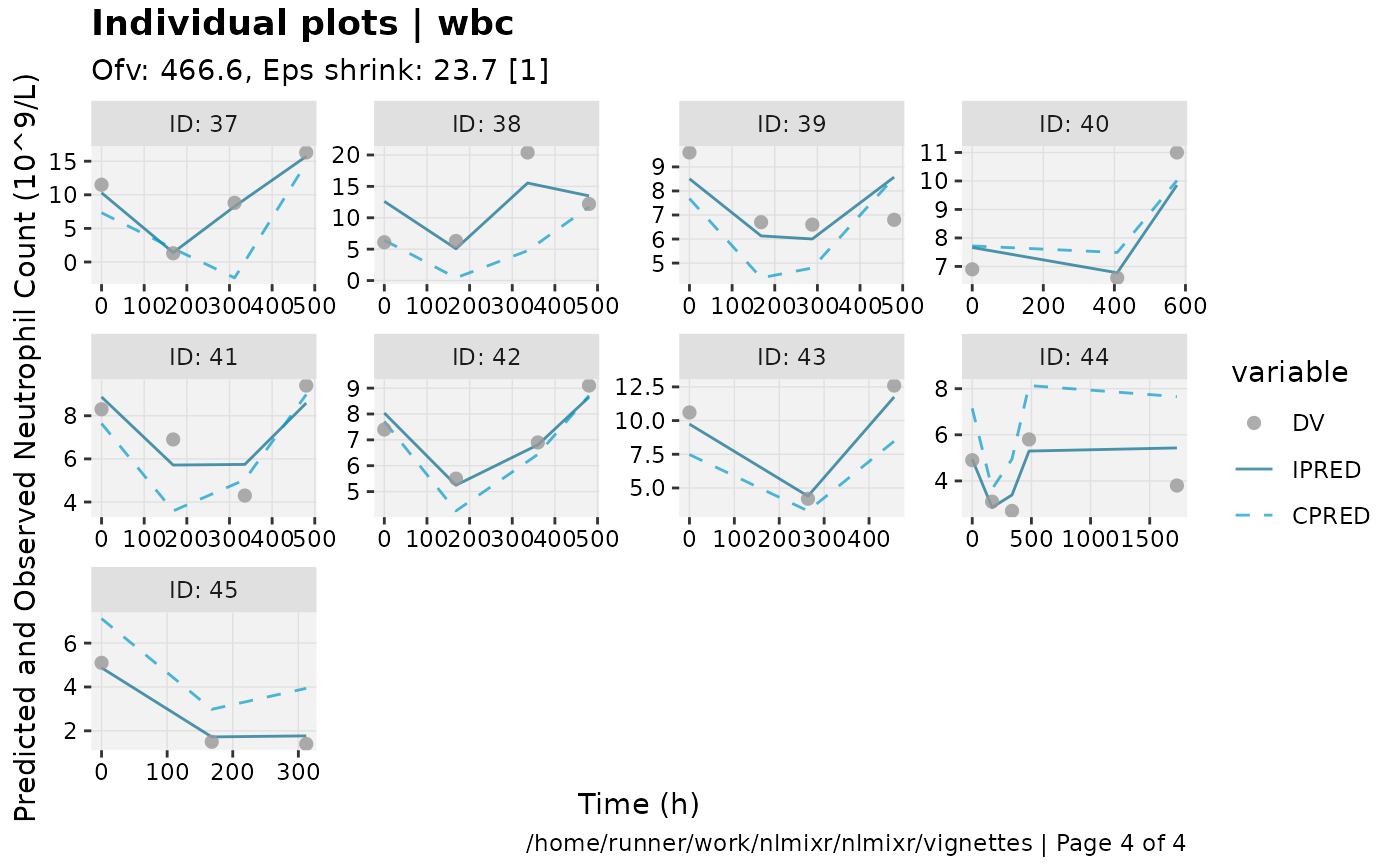
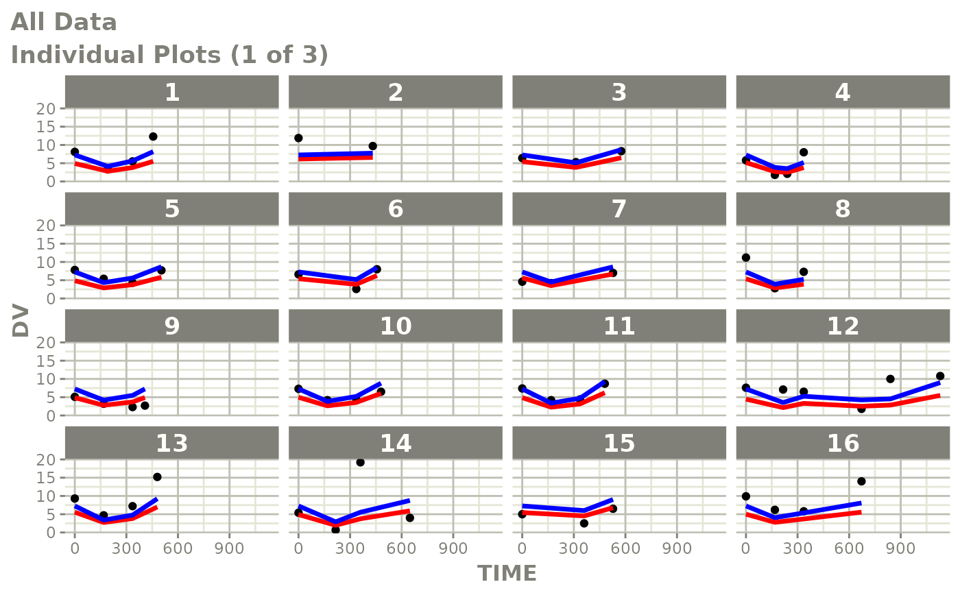
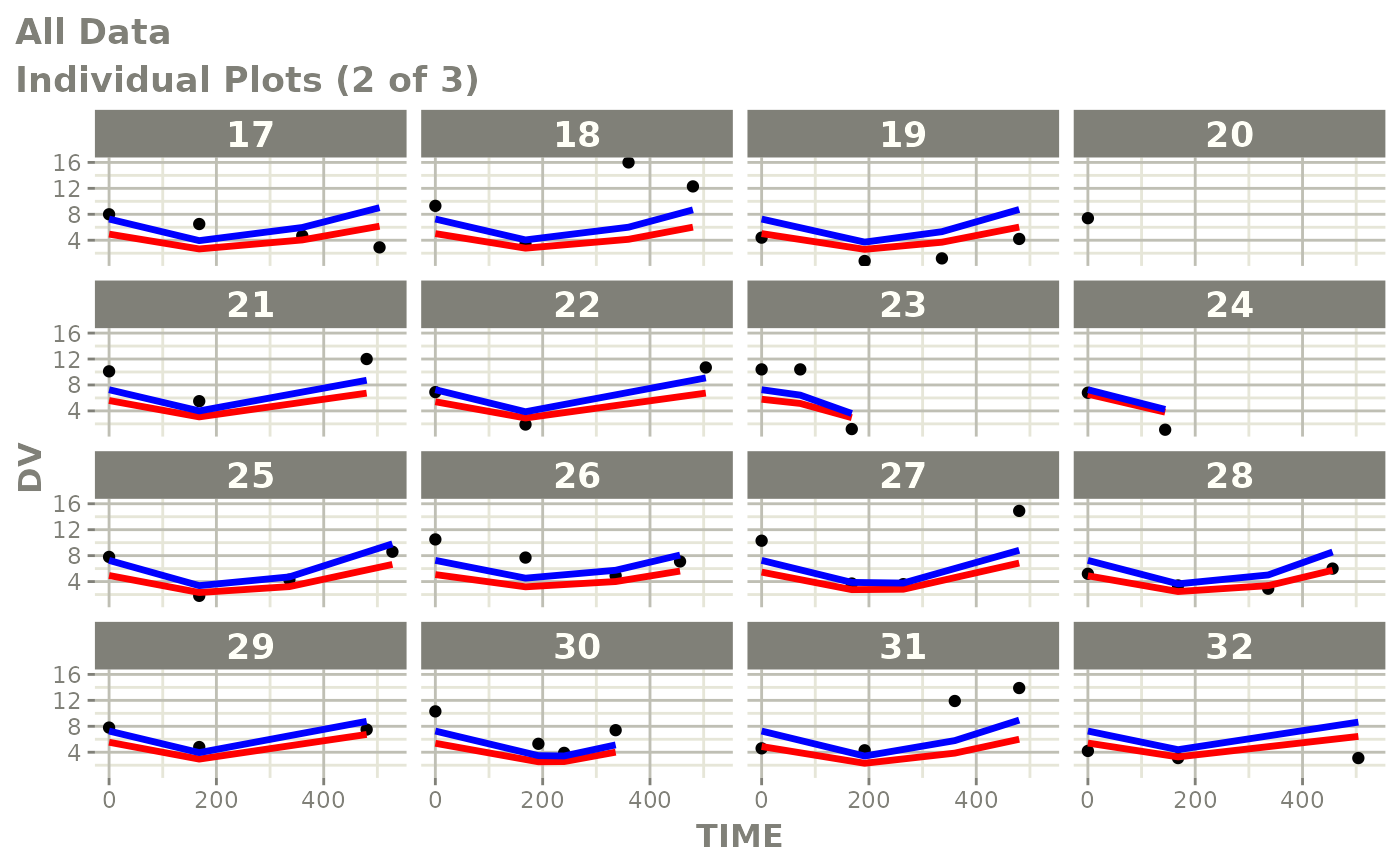
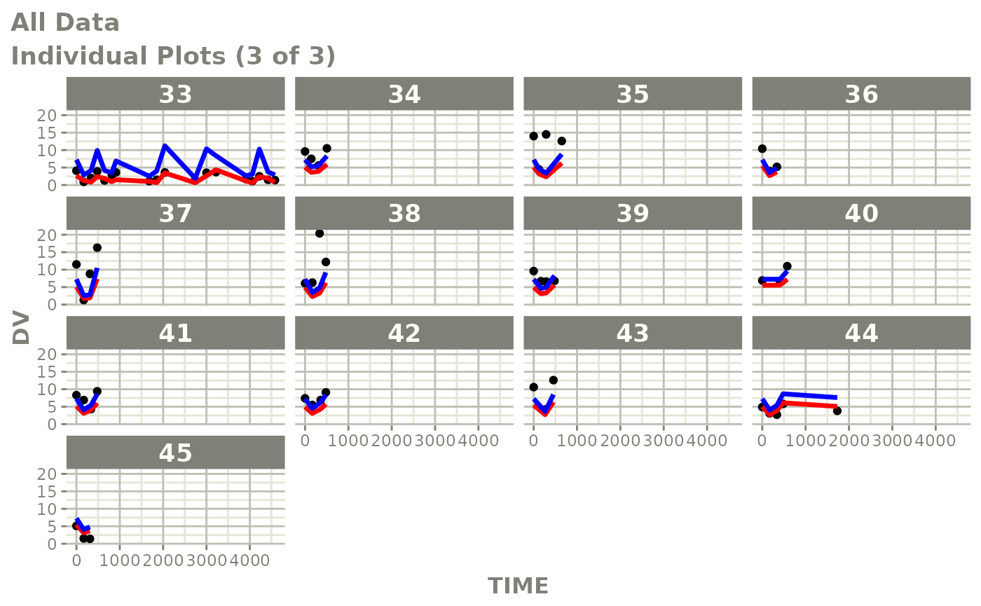
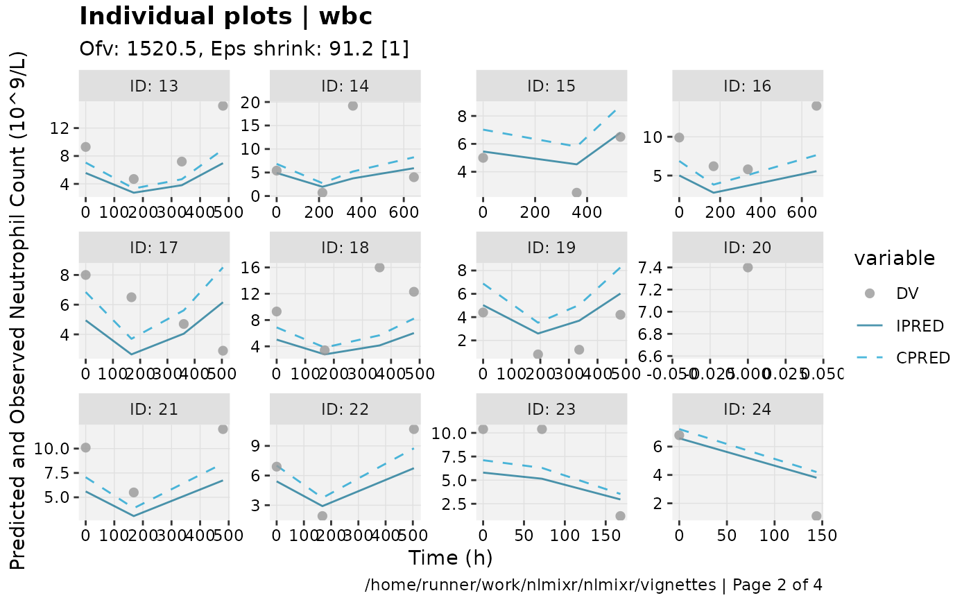
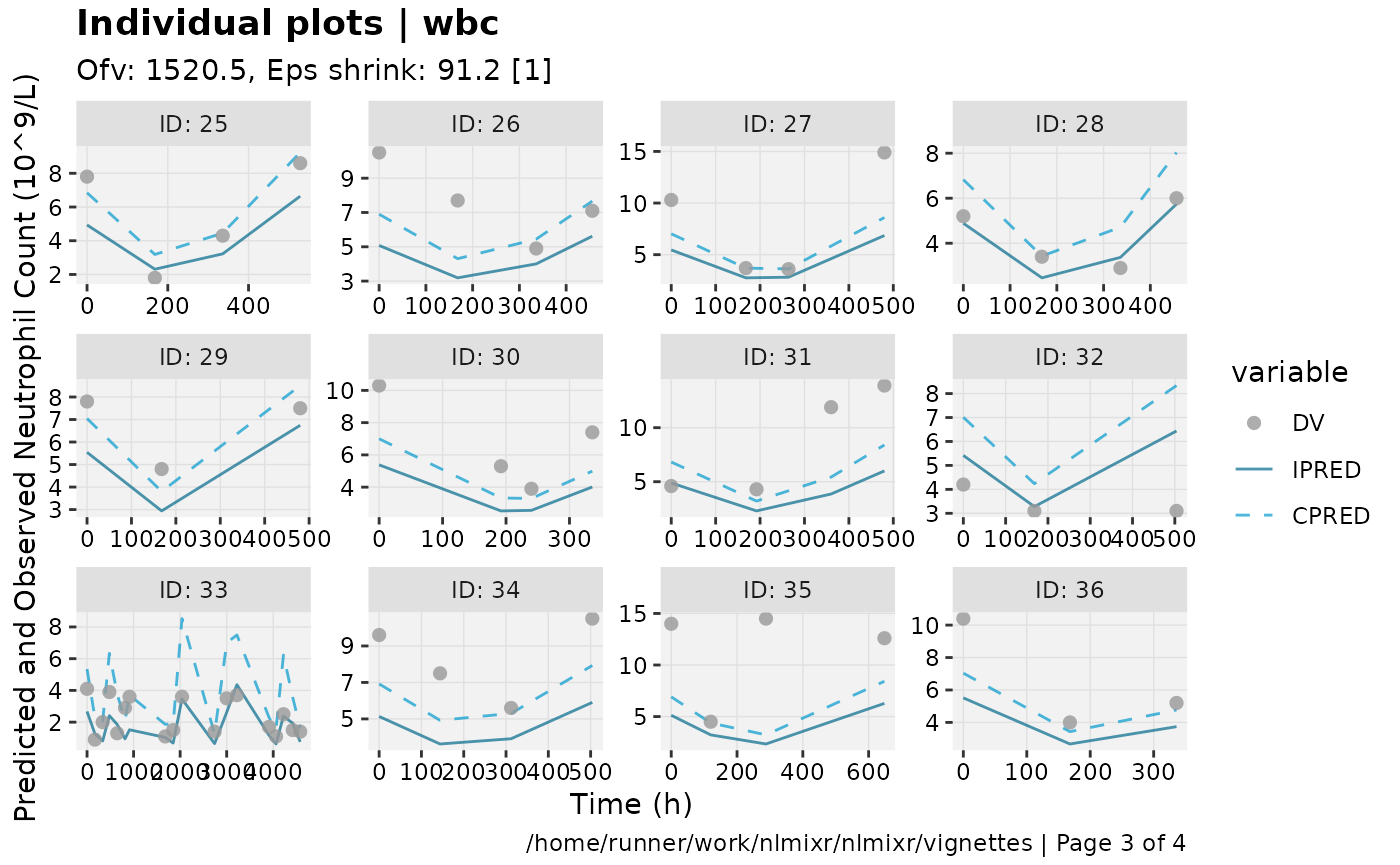
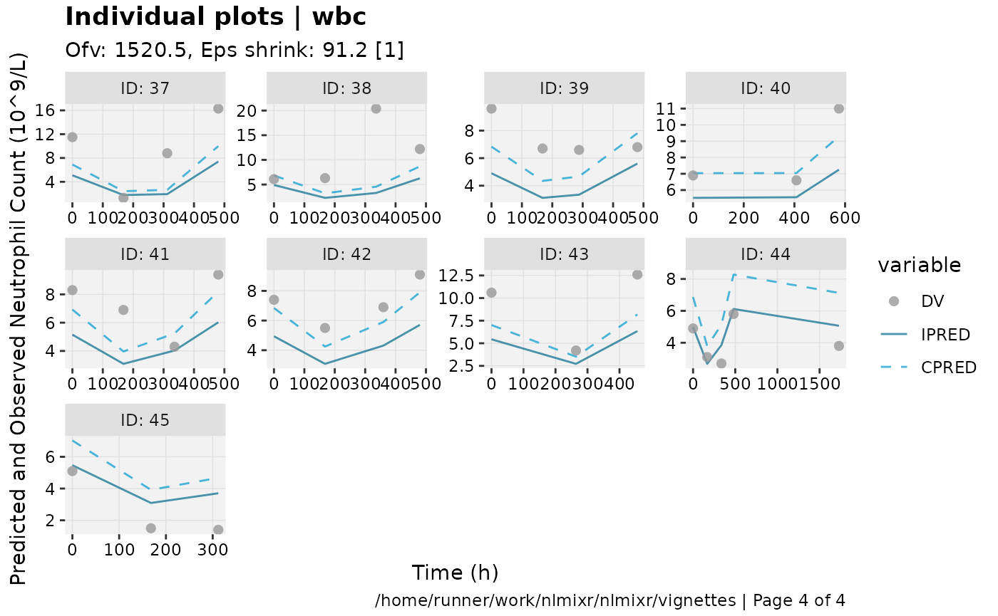
print(ind_plots(xpdb, nrow=3, ncol=4) +
      ylab("Predicted and Observed Neutrophil Count (10^9/L)") +
      xlab("Time (h)"))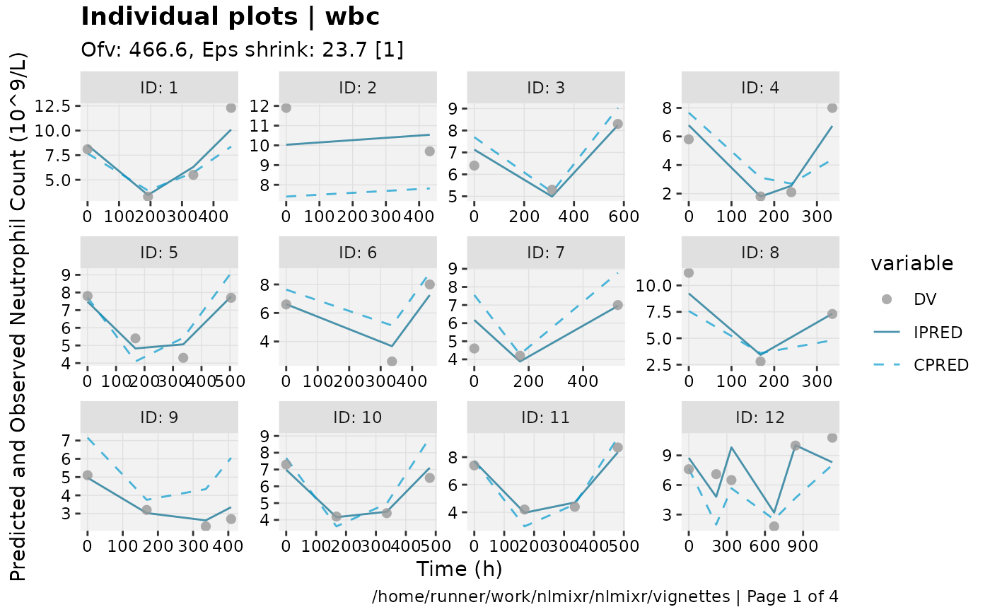


print(res_distrib(xpdb) +
      ylab("Density") +
      xlab("Conditional Weighted Residuals"))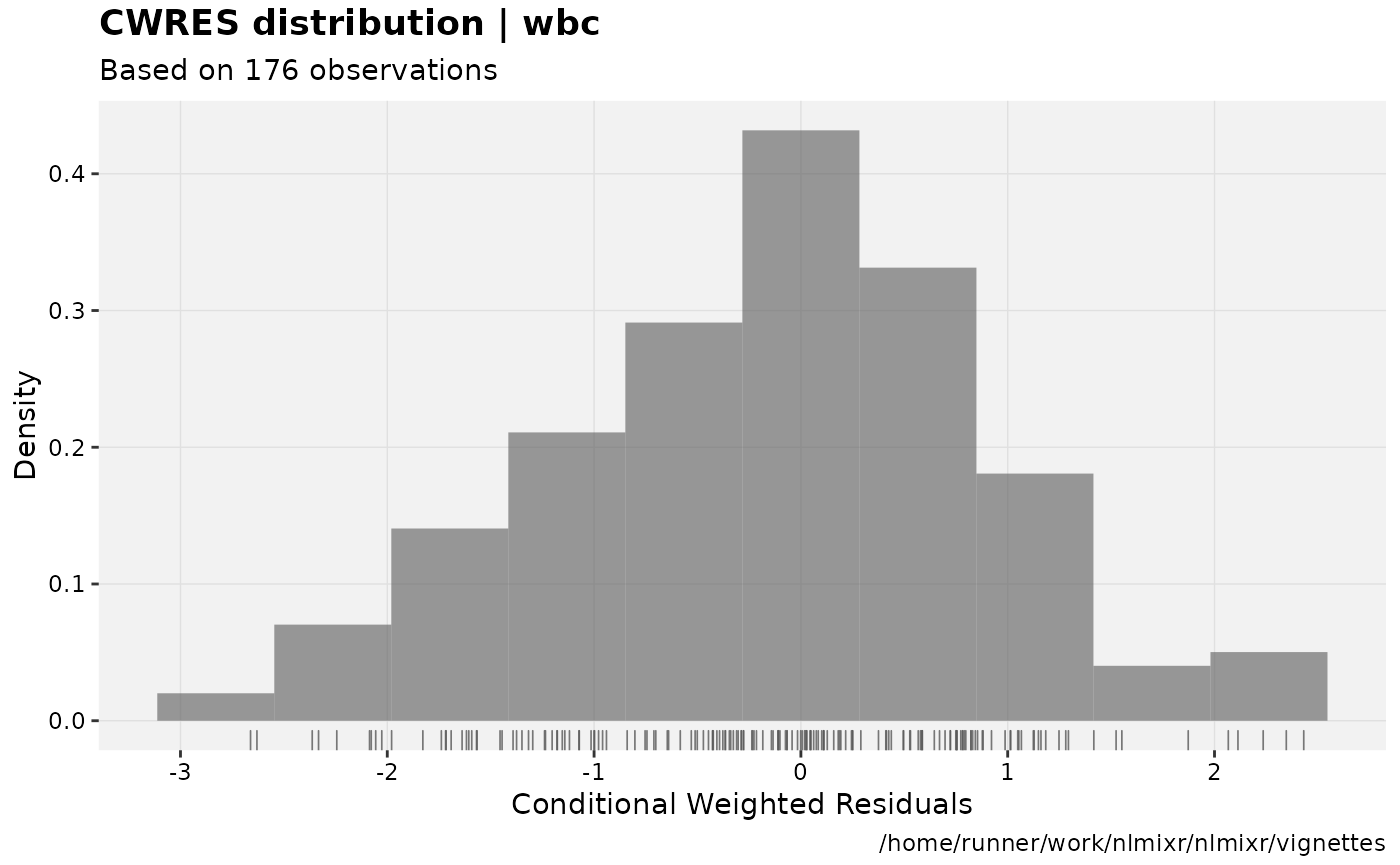


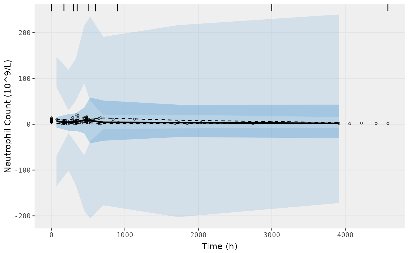
vpc.ui(fit.S, n=500, n_bins = 10, show=list(obs_dv=T), ylab = "Neutrophil Count (10^9/L)", xlab = "Time (h)")
#> [====|====|====|====|====|====|====|====|====|====] 0:00:07
#>   $rxsim = original simulated data
#>   $sim = merge simulated data
#>   $obs = observed data
#>   $gg = vpc ggplot
#> use vpc(...) to change plot options
#> plotting the object now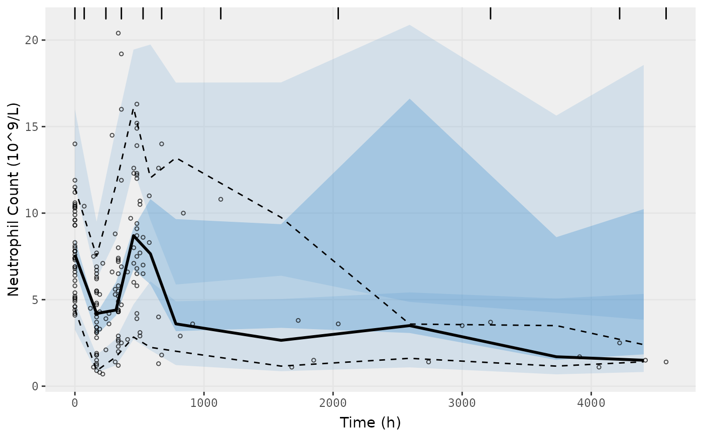


vpc.ui(fit.S, n=500, bins = c(0,170,300,350,500,600,900,3000,4580), show=list(obs_dv=T), ylab = "Neutrophil Count (10^9/L)", xlab = "Time (h)")
#> [====|====|====|====|====|====|====|====|====|====] 0:00:07
#>   $rxsim = original simulated data
#>   $sim = merge simulated data
#>   $obs = observed data
#>   $gg = vpc ggplot
#> use vpc(...) to change plot options
#> plotting the object now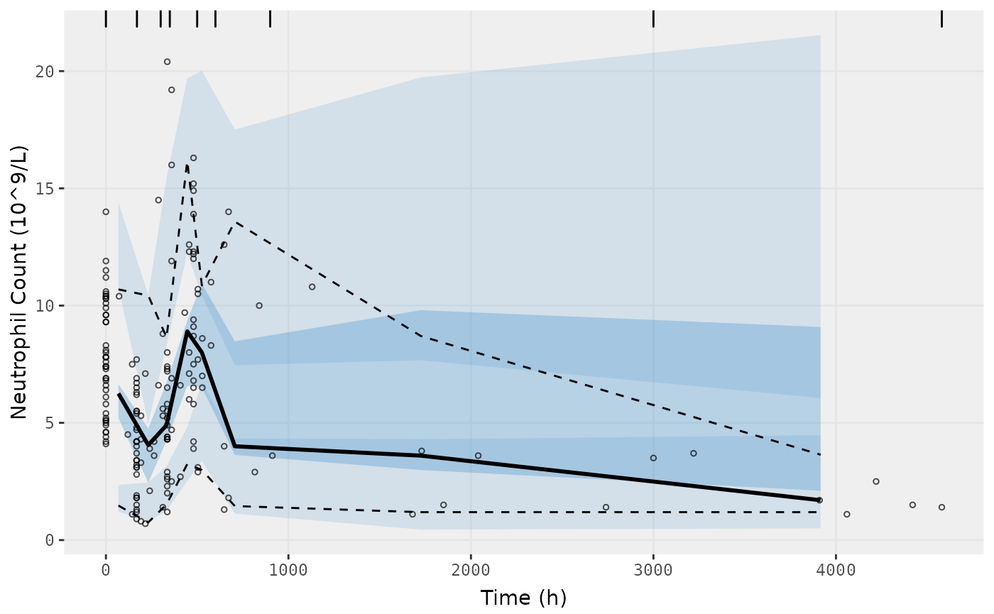

Fit model using FOCEi

fit.F <- nlmixr(wbc, d3, est="focei", list(print=0), table=list(cwres=TRUE, npde=TRUE))
#> [====|====|====|====|====|====|====|====|====|====] 0:00:00 
#> 
#> [====|====|====|====|====|====|====|====|====|====] 0:00:00 
#> 
#> [====|====|====|====|====|====|====|====|====|====] 0:00:00 
#> 
#> [====|====|====|====|====|====|====|====|====|====] 0:00:00 
#> 
#> [====|====|====|====|====|====|====|====|====|====] 0:00:00 
#> 
#> [====|====|====|====|====|====|====|====|====|====] 0:00:00 
#> 
#> [====|====|====|====|====|====|====|====|====|====] 0:00:00 
#> 
#> [====|====|====|====|====|====|====|====|====|====] 0:00:00 
#> 
#> [====|====|====|====|====|====|====|====|====|====] 0:00:00 
#> 
#> [====|====|====|====|====|====|====|====|====|====] 0:00:00 
#> 
#> [1] "V2I" "CLI" "V1I"
#> unhandled error message: EE:[lsoda] 500000 steps taken before reaching tout
#>  @(lsoda.c:750
#> calculating covariance matrix
#> [====|====|====|====|====|====|====|====|===
S matrix calculation failed; Switch to R-matrix covariance.
#> =|====] 0:00:34 
#> done
#> [====|====|====|====|====|====|====|====|====|====] 0:00:03

FOCEi Goodness of fit plots

xpdb <- xpose_data_nlmixr(fit.F)
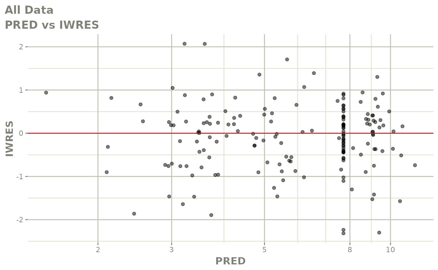
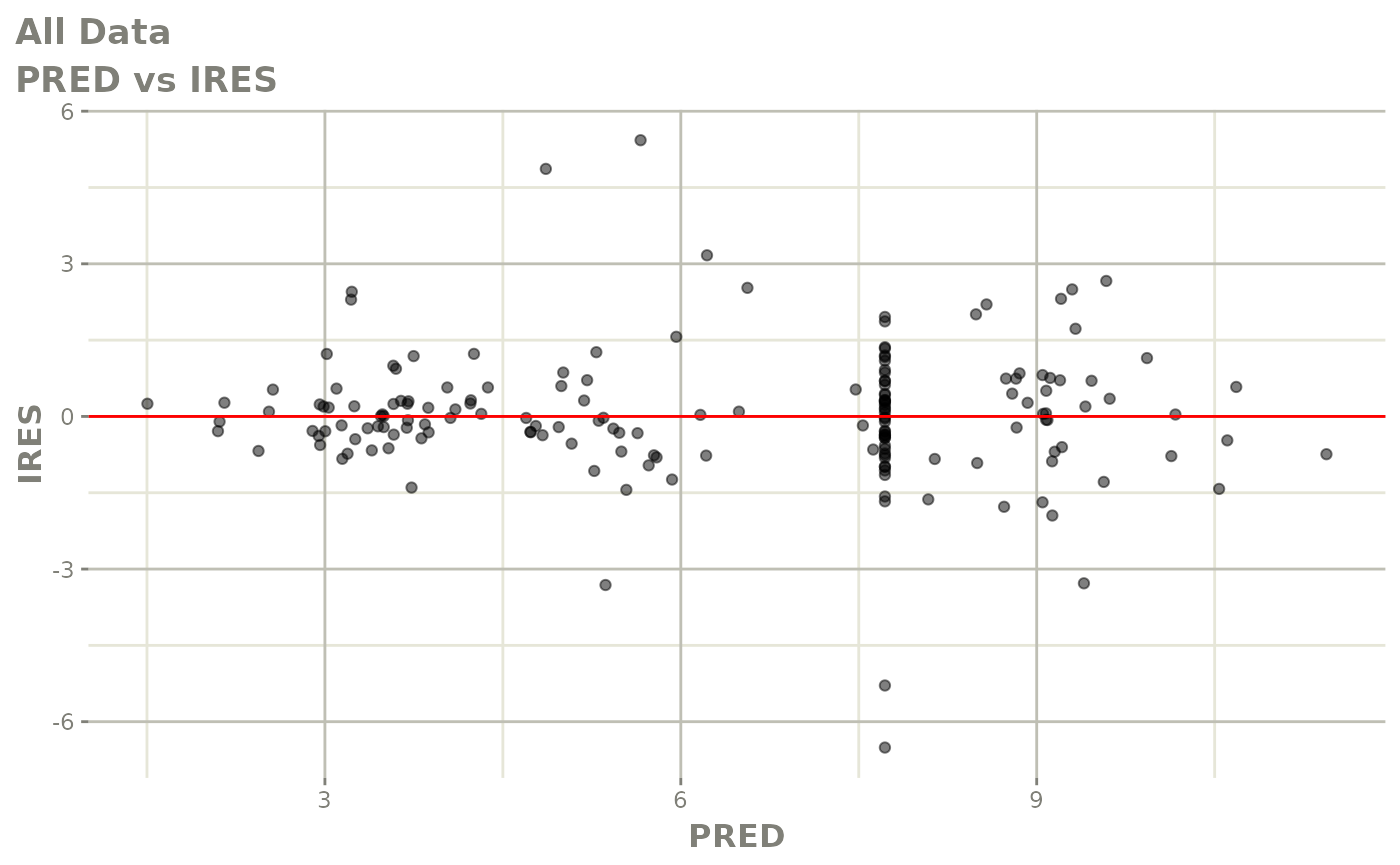
plot(fit.F)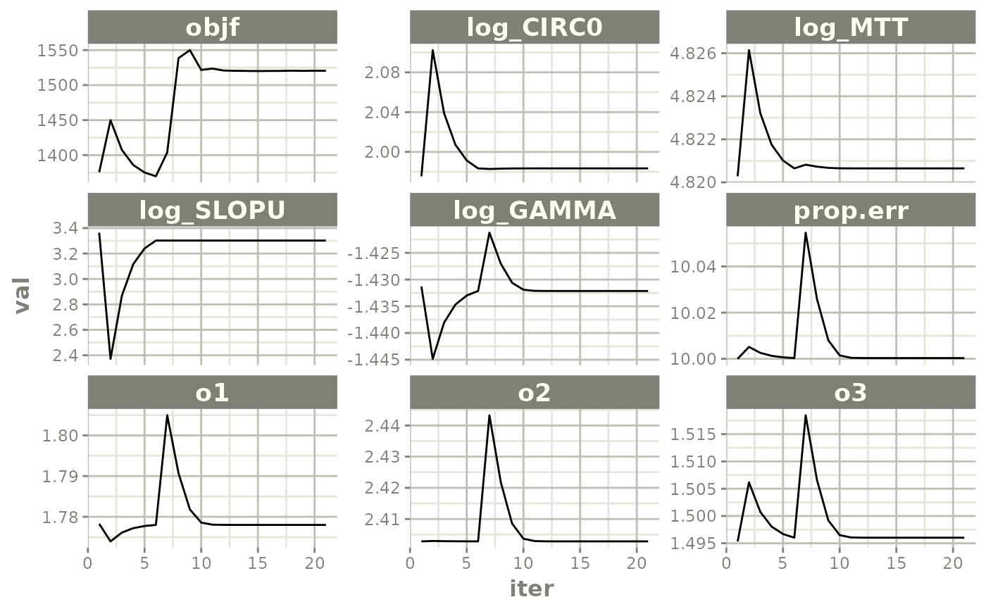

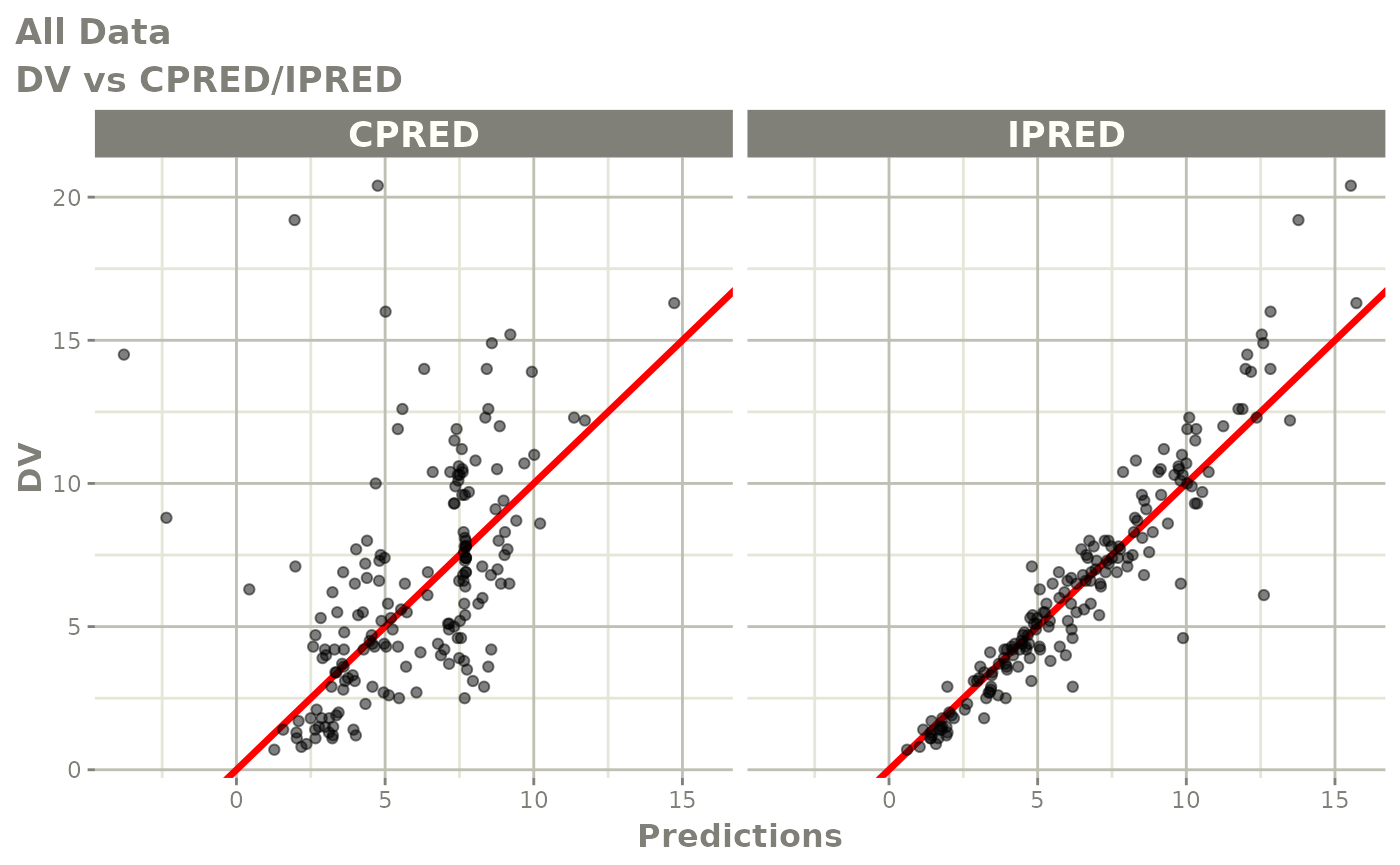
print(dv_vs_pred(xpdb) +
      ylab("Observed Neutrophil Count (10^9/L)") +
      xlab("Population Predicted Neutrophil Count (10^9/L)"))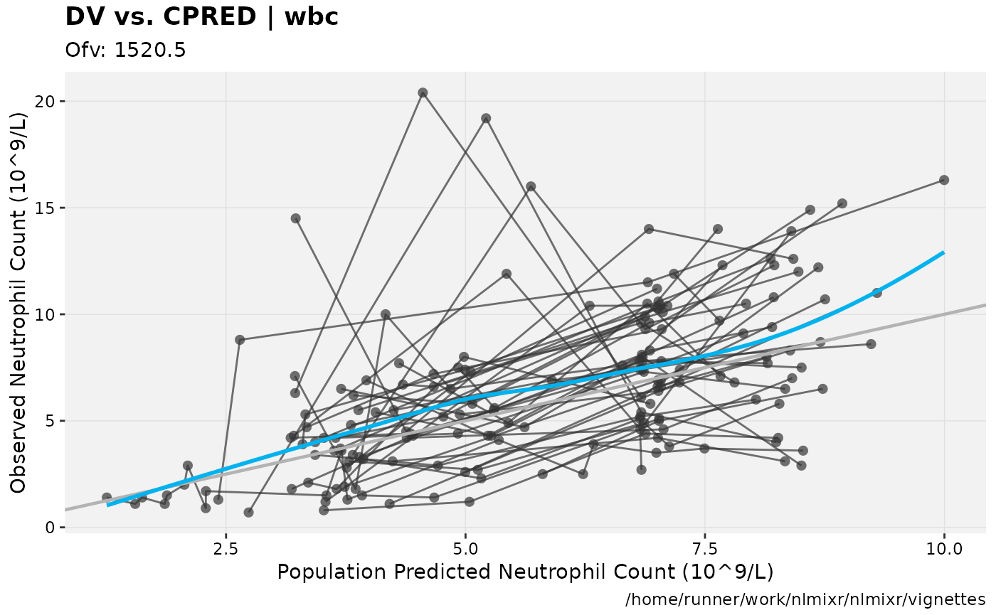


print(dv_vs_ipred(xpdb) +
      ylab("Observed Neutrophil Count (10^9/L)") +
      xlab("Individual Predicted Neutrophil Count (10^9/L)"))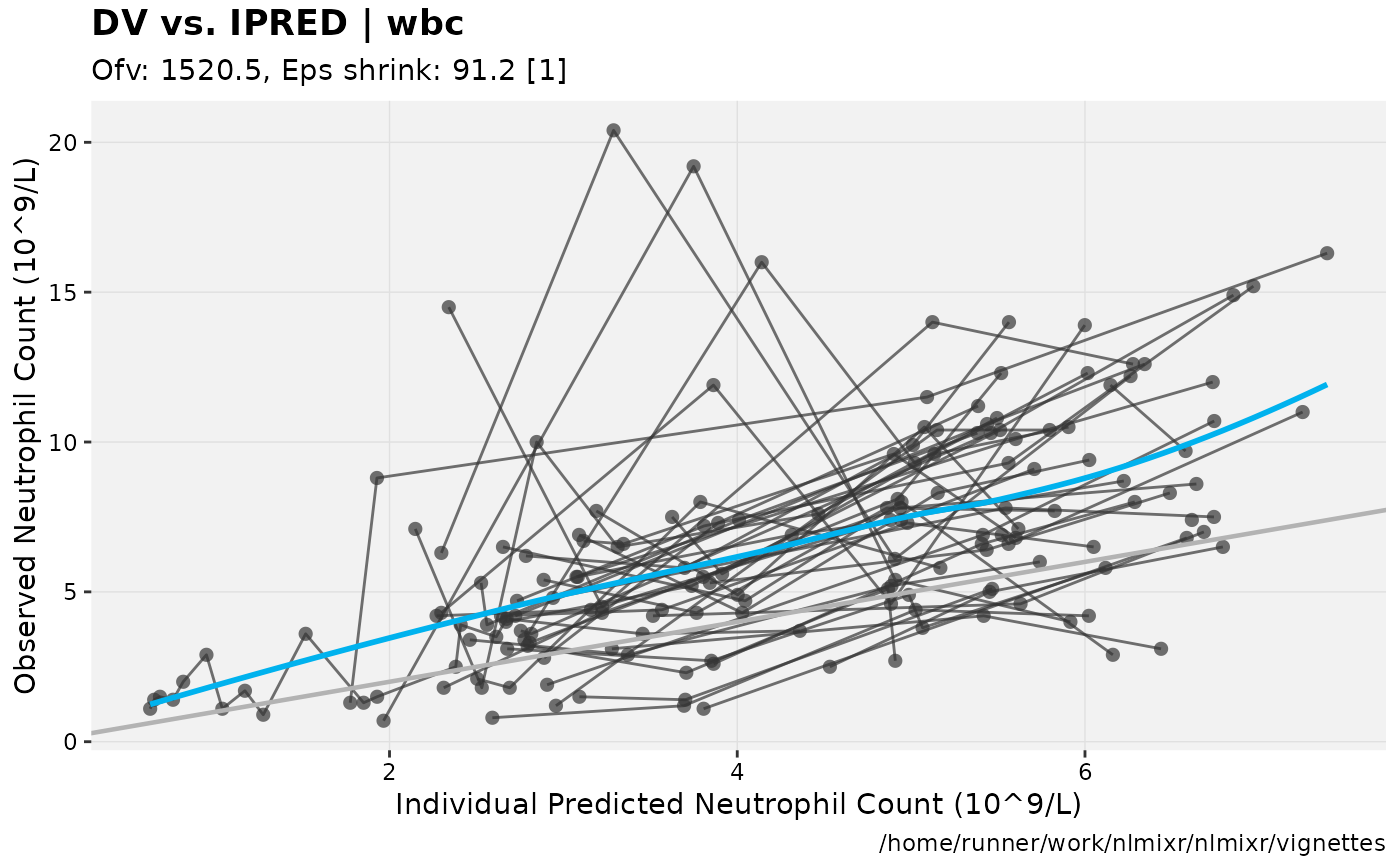


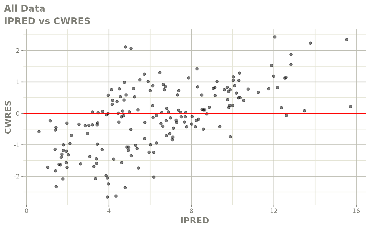
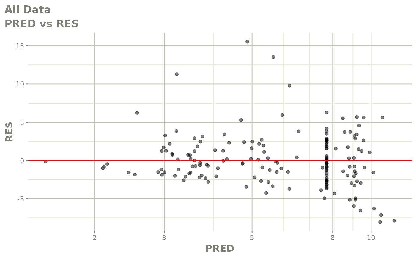
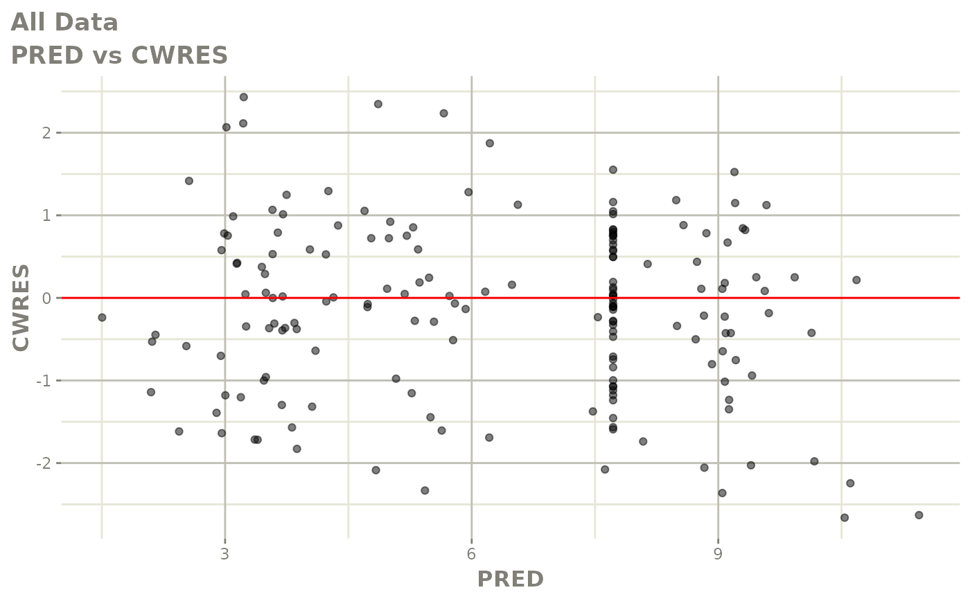
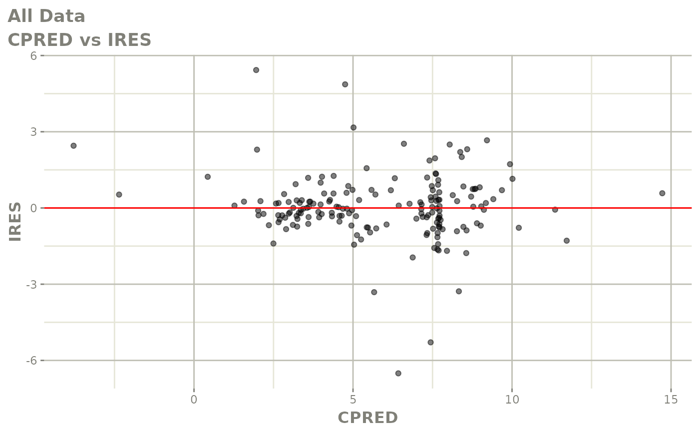
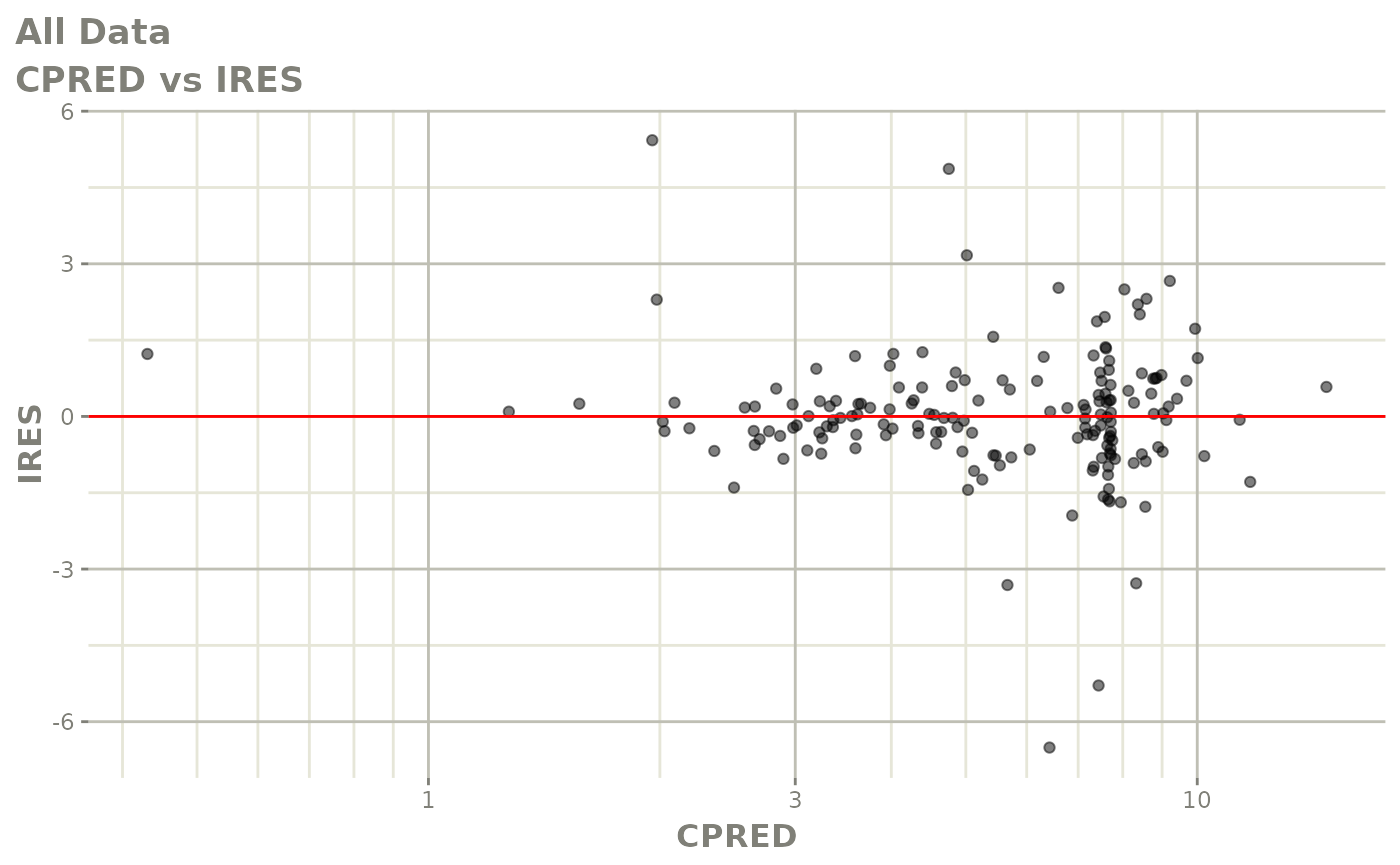
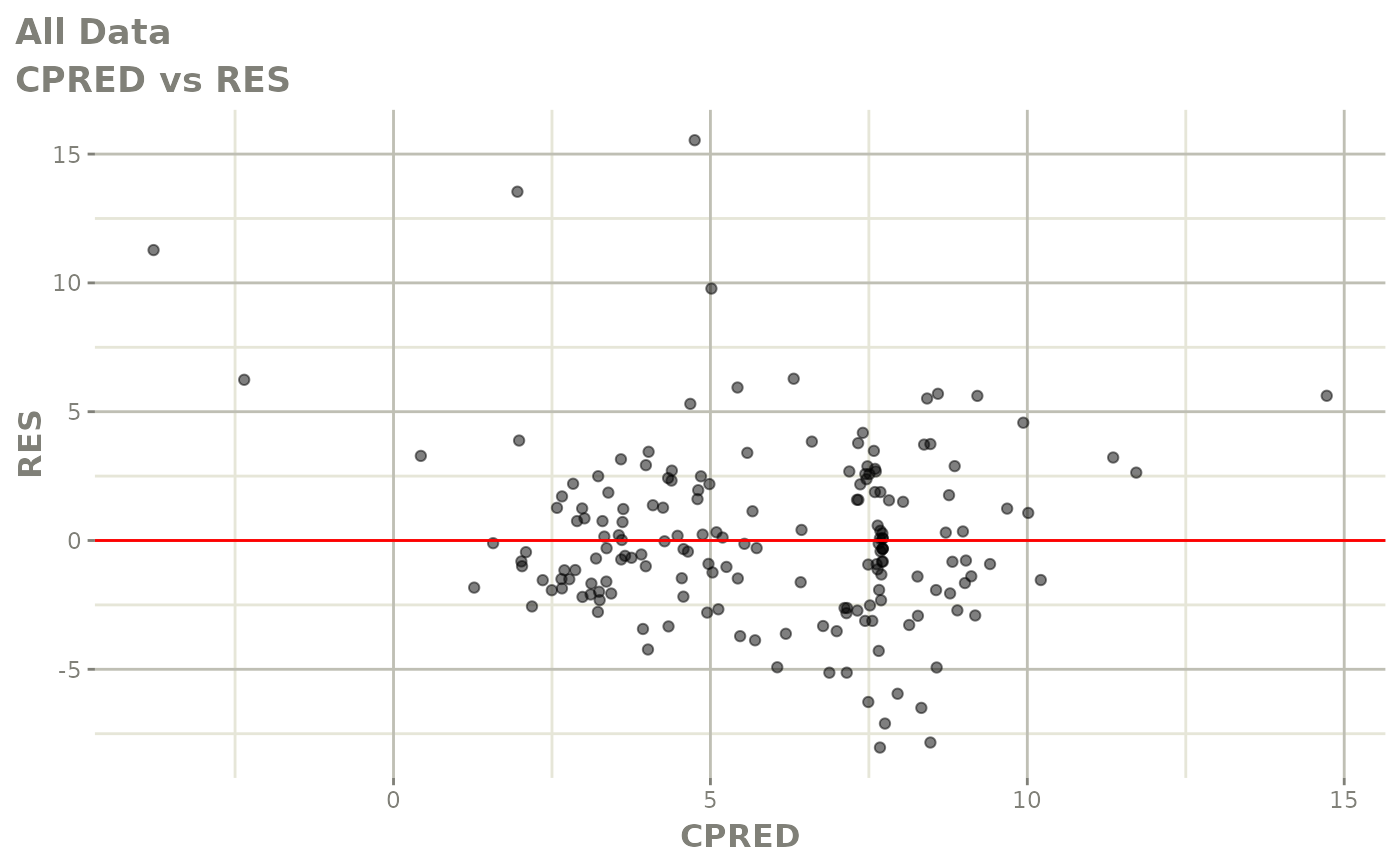
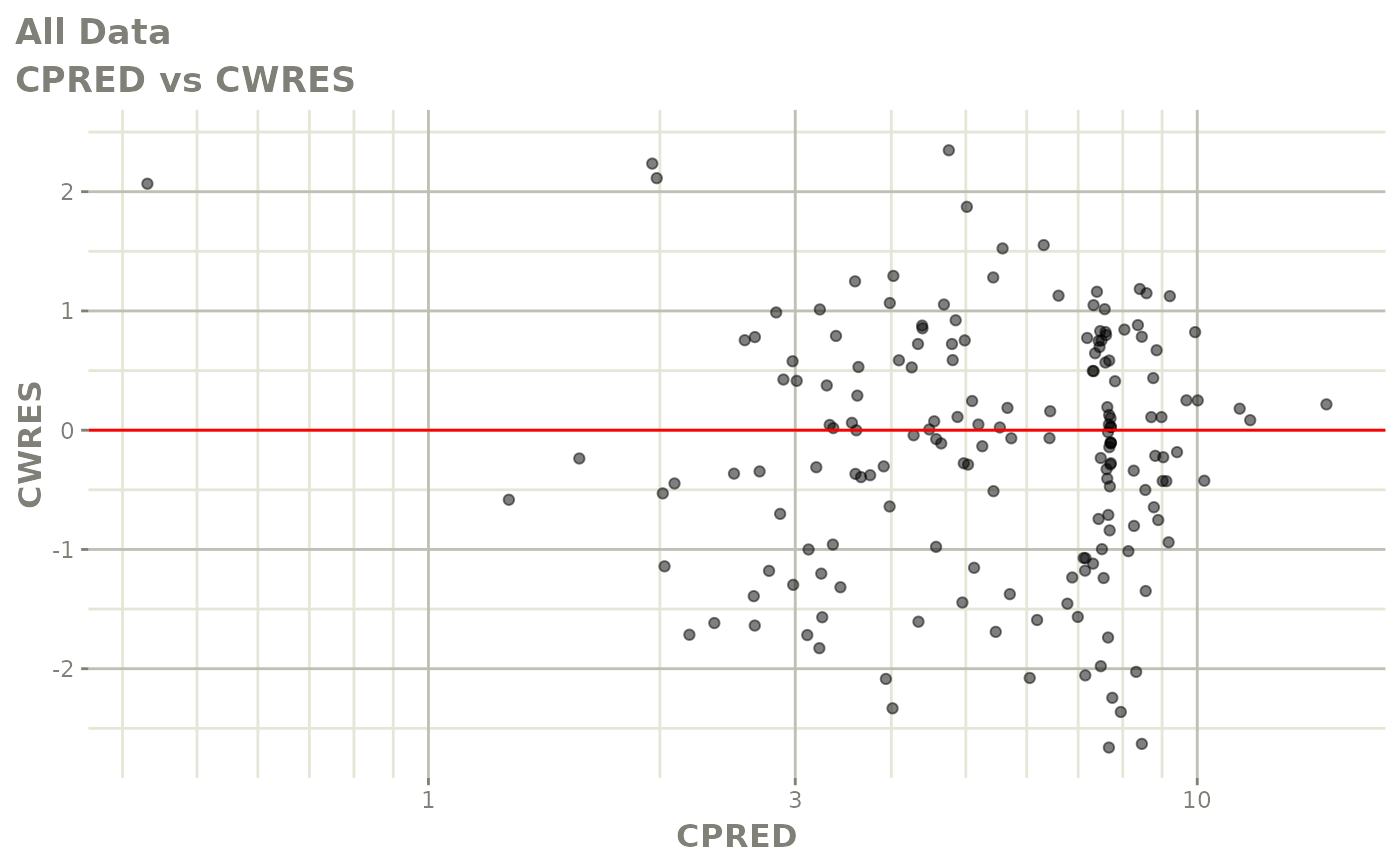
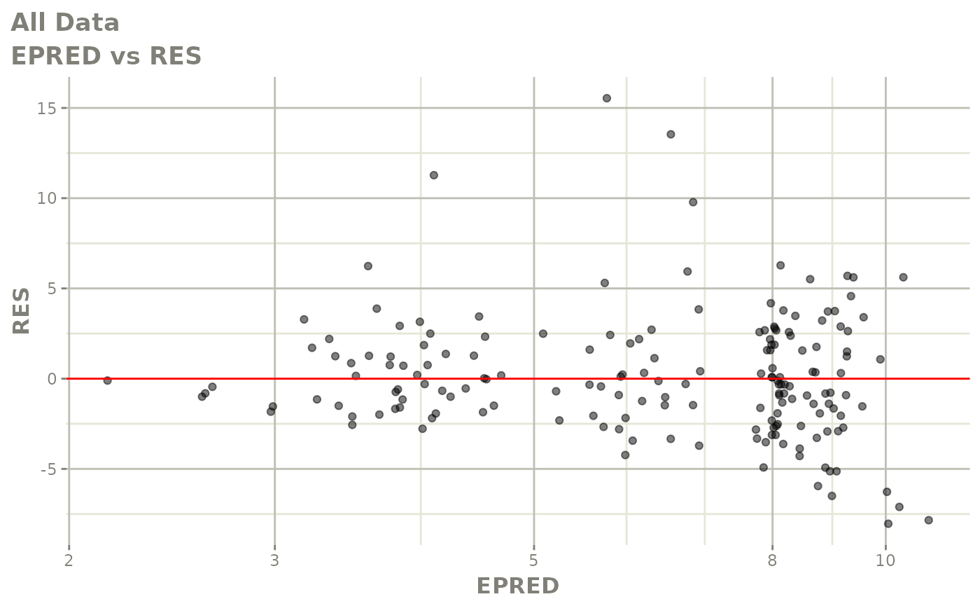
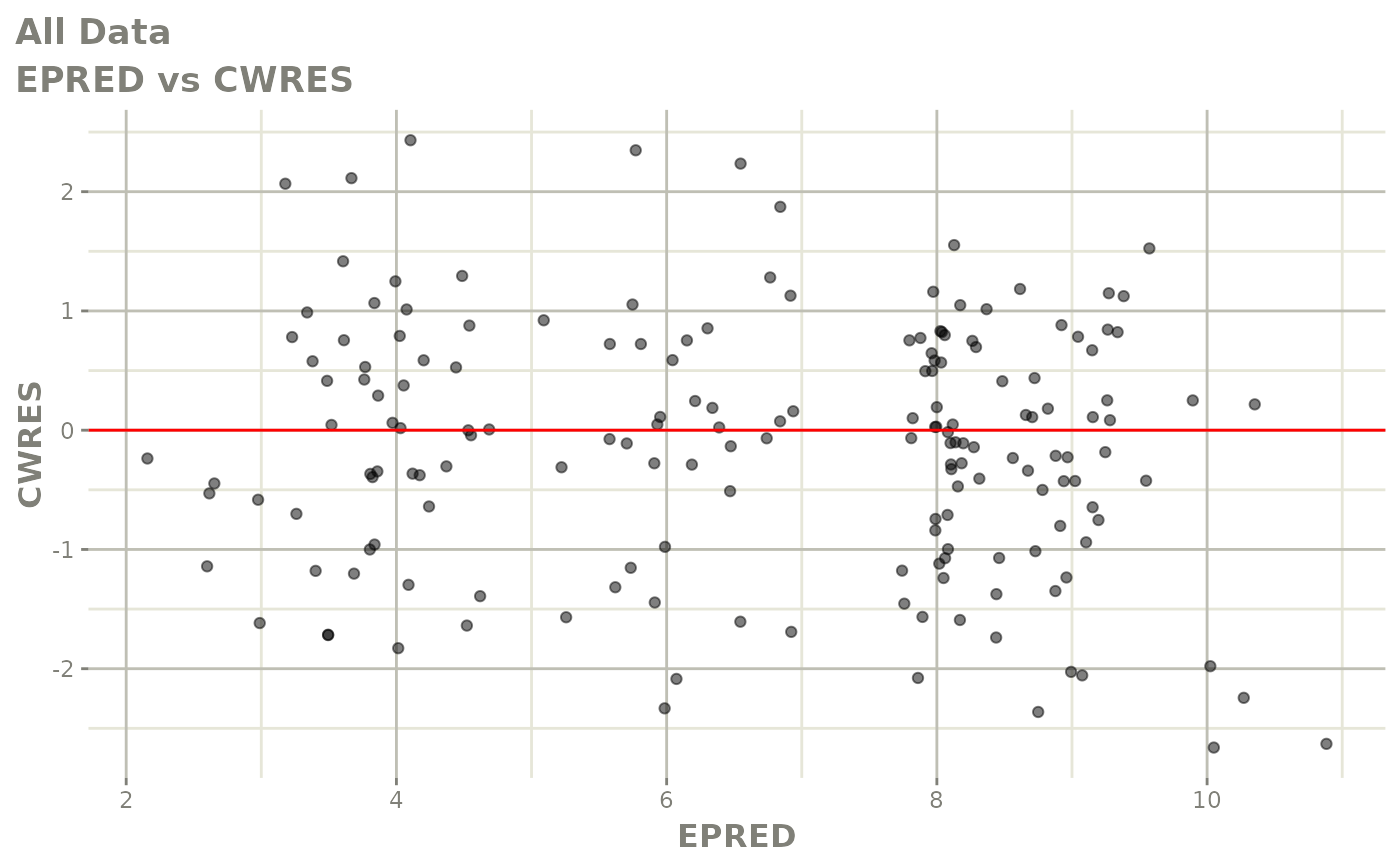
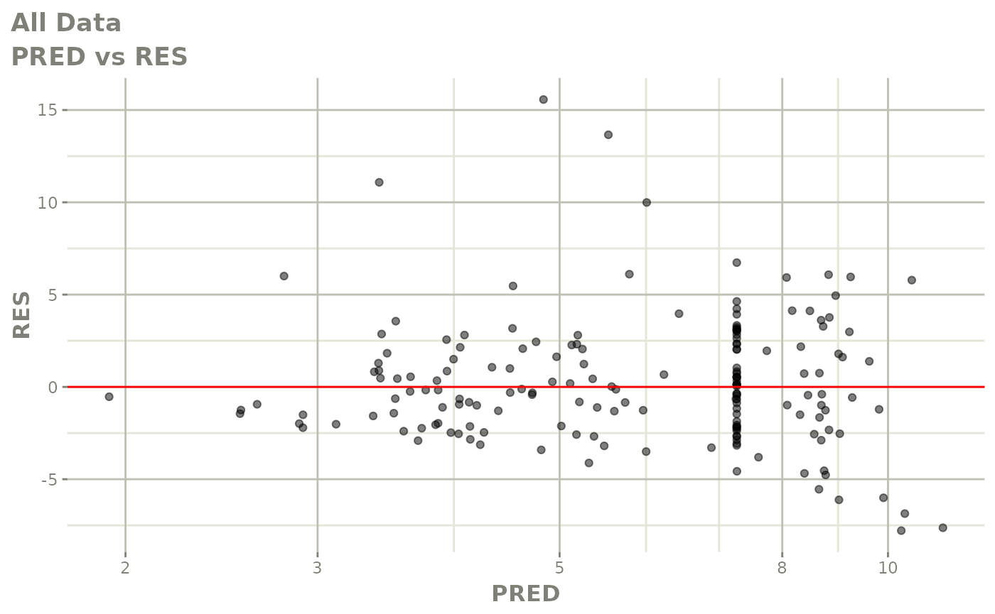
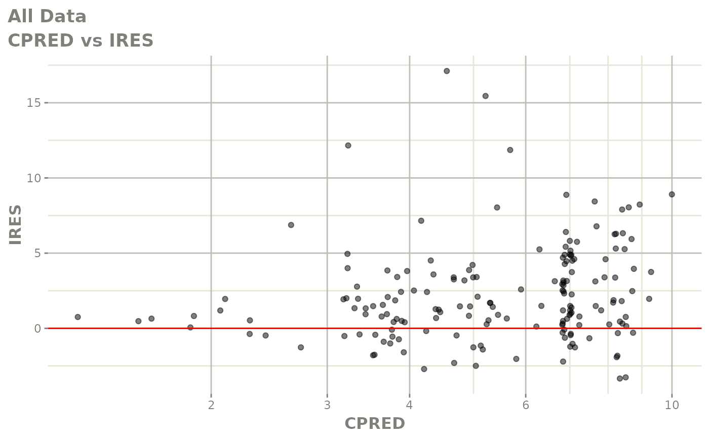
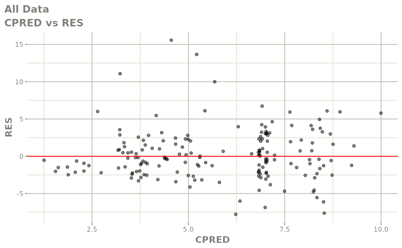
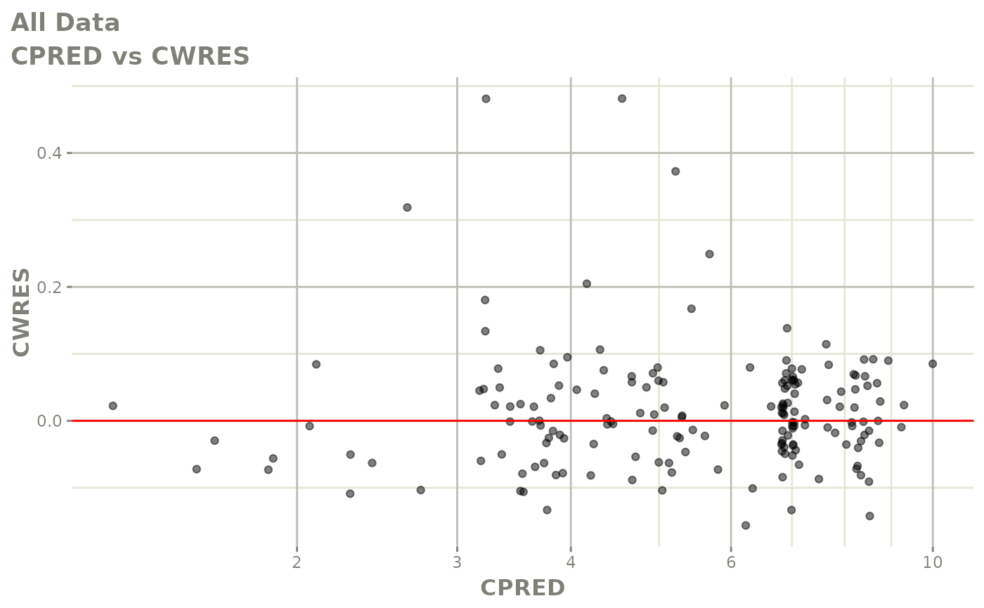
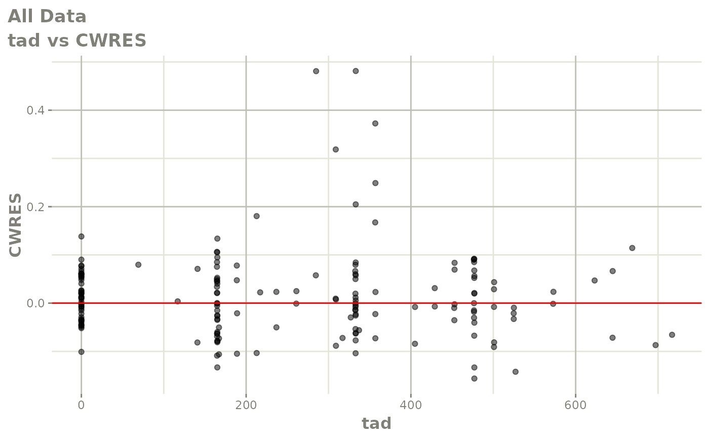
print(res_vs_pred(xpdb) +
      ylab("Conditional Weighted Residuals") +
      xlab("Population Predicted Neutrophil Count (10^9/L)"))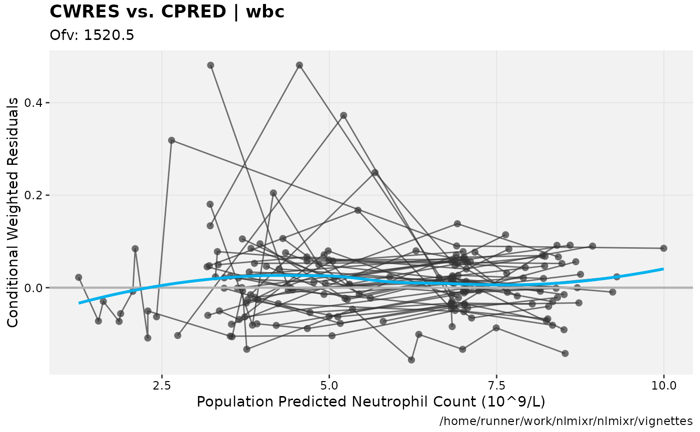


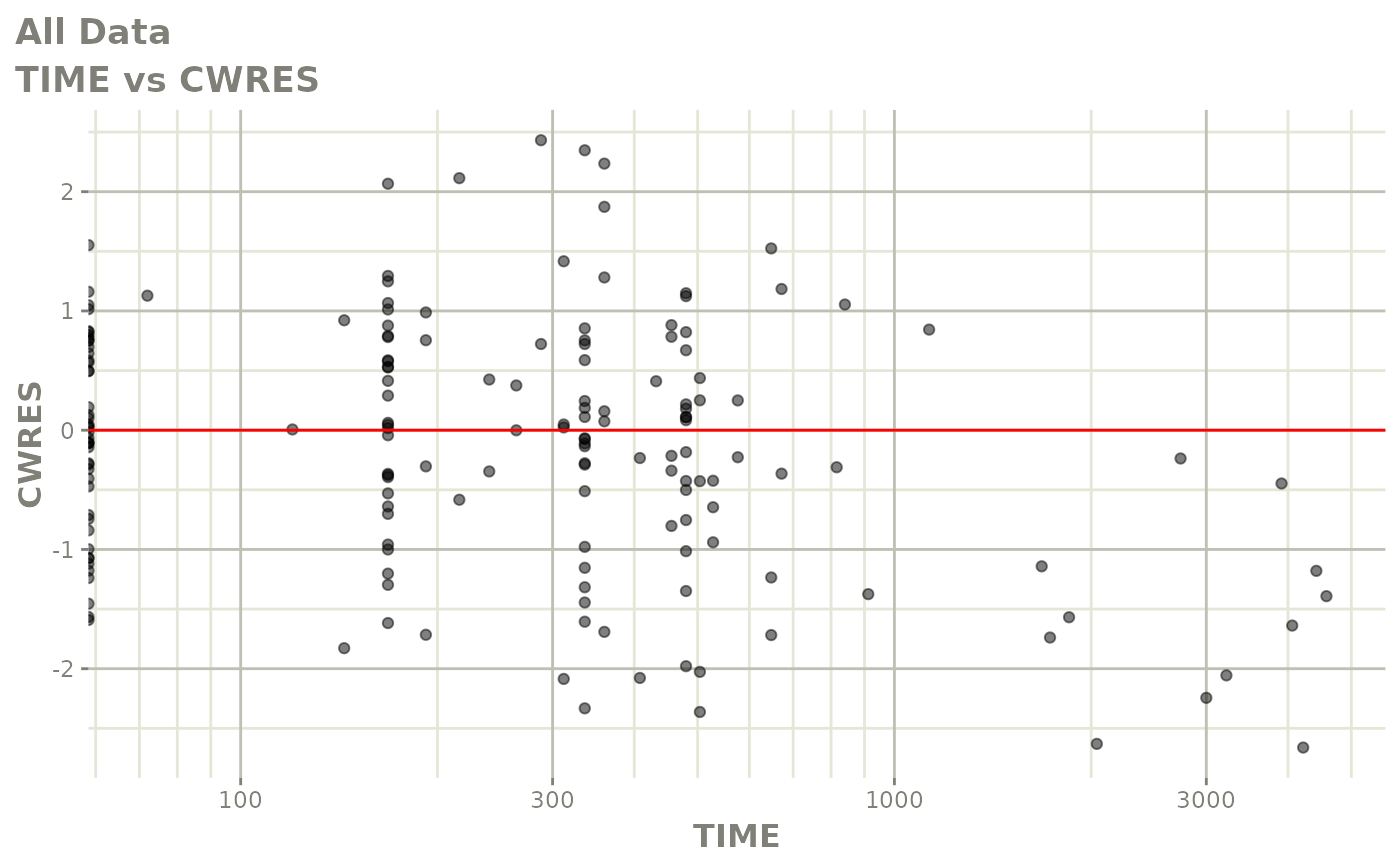
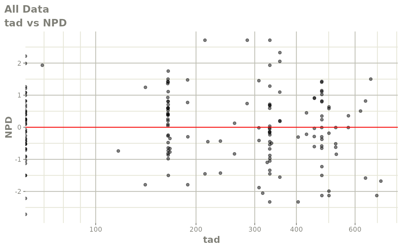
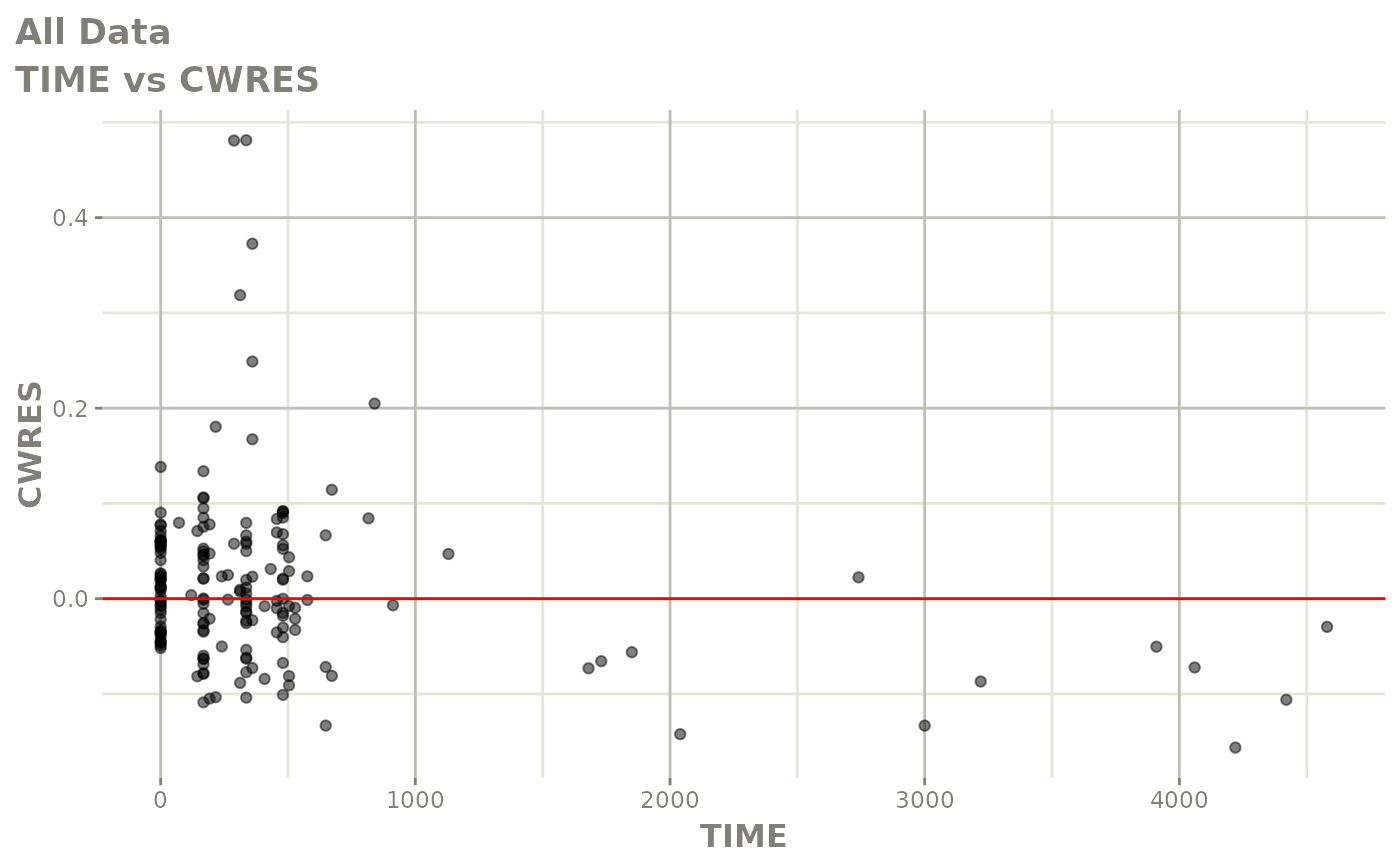
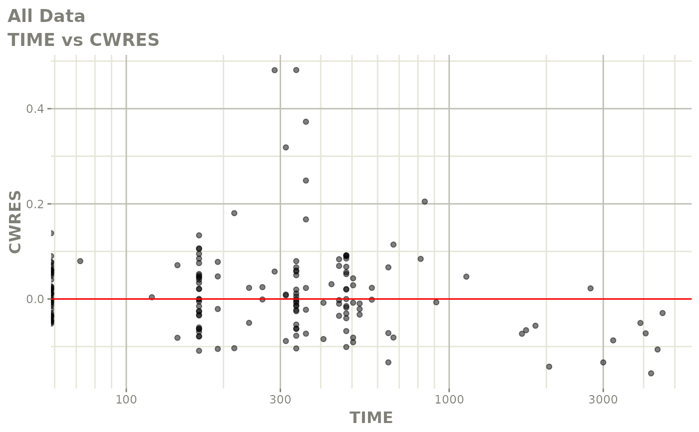
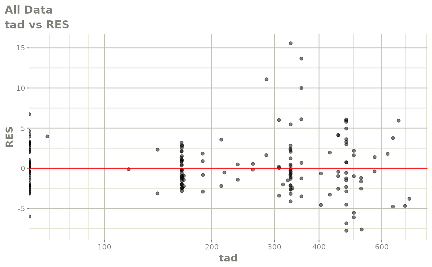
print(res_vs_idv(xpdb) +
      ylab("Conditional Weighted Residuals") +
      xlab("Time (h)"))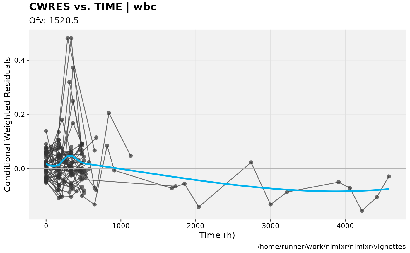


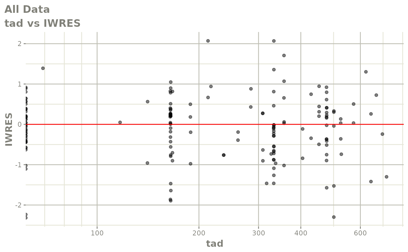
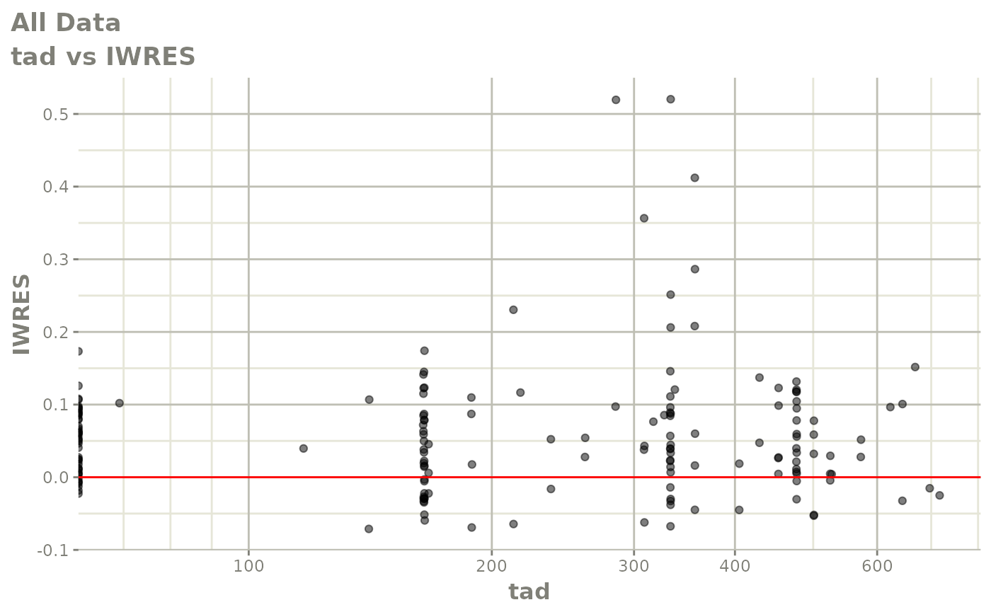
print(absval_res_vs_idv(xpdb, res = 'IWRES') +
      ylab("Individual Weighted Residuals") +
      xlab("Time (h)"))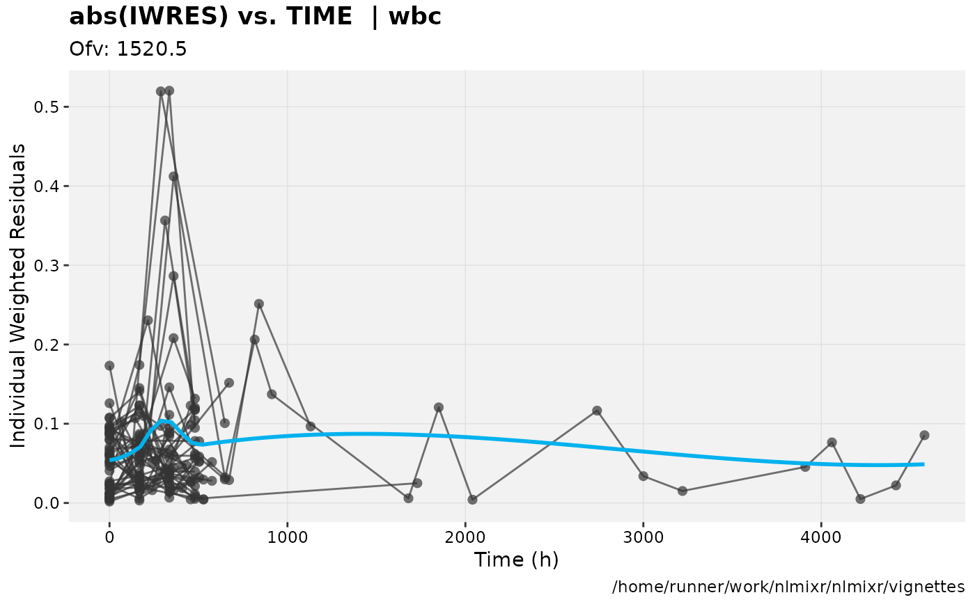


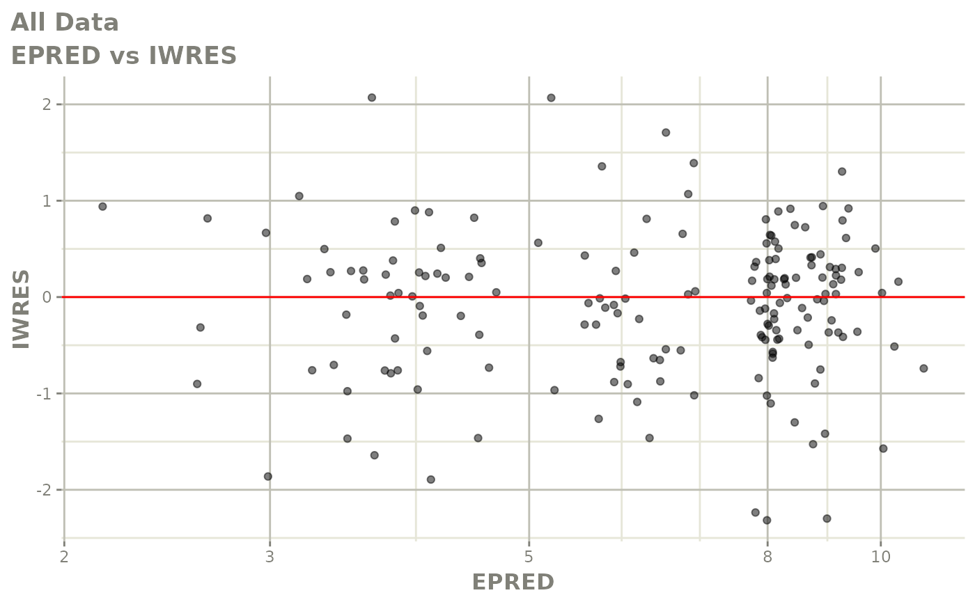
print(absval_res_vs_pred(xpdb, res = 'IWRES') +
      ylab("Individual Weighted Residuals") +
      xlab("Population Predicted Neutrophil Count (10^9/L)"))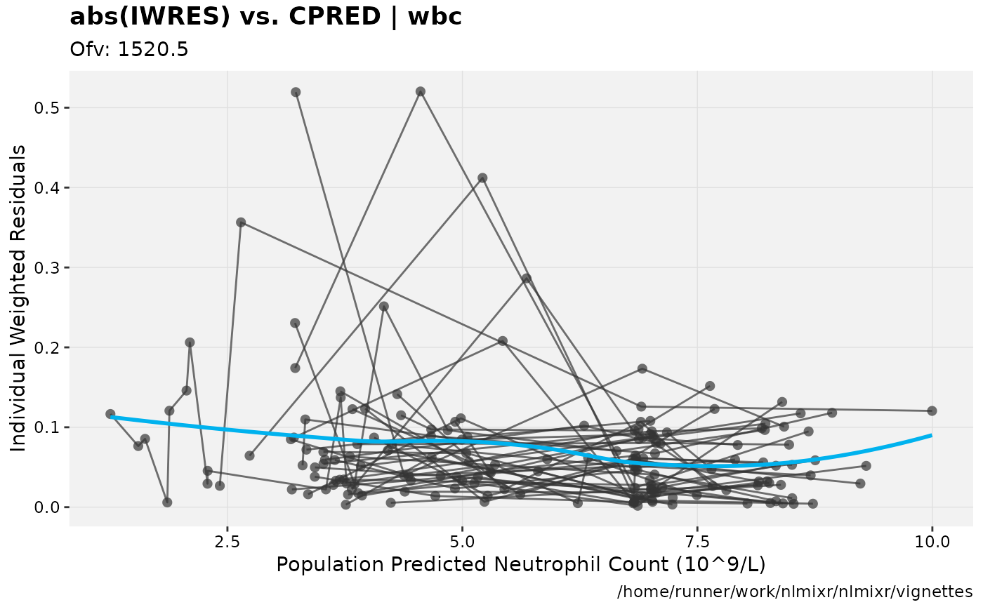


print(ind_plots(xpdb, nrow=3, ncol=4) +
      ylab("Predicted and Observed Neutrophil Count (10^9/L)") +
      xlab("Time (h)"))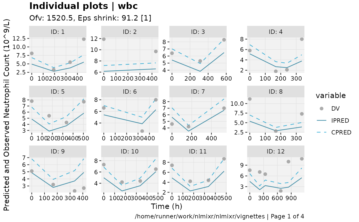


print(res_distrib(xpdb) +
      ylab("Density") +
      xlab("Conditional Weighted Residuals"))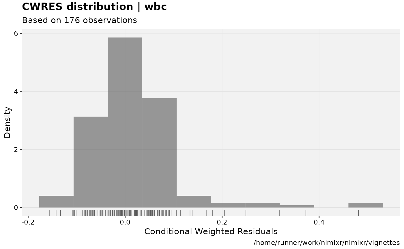


#vpc.ui(fit.S, n=500, show=list(obs_dv=T), ylab = "Neutrophil count (10^9/L)", xlab = "Time (h)")
# 10 bins is slightly better than auto bin
vpc.ui(fit.F, n=500, n_bins = 10, show=list(obs_dv=T), ylab = "Neutrophil Count (10^9/L)", xlab = "Time (h)")
#> [====|====|====|====|====|====|====|====|====|====] 0:00:05
#>   $rxsim = original simulated data
#>   $sim = merge simulated data
#>   $obs = observed data
#>   $gg = vpc ggplot
#> use vpc(...) to change plot options
#> plotting the object now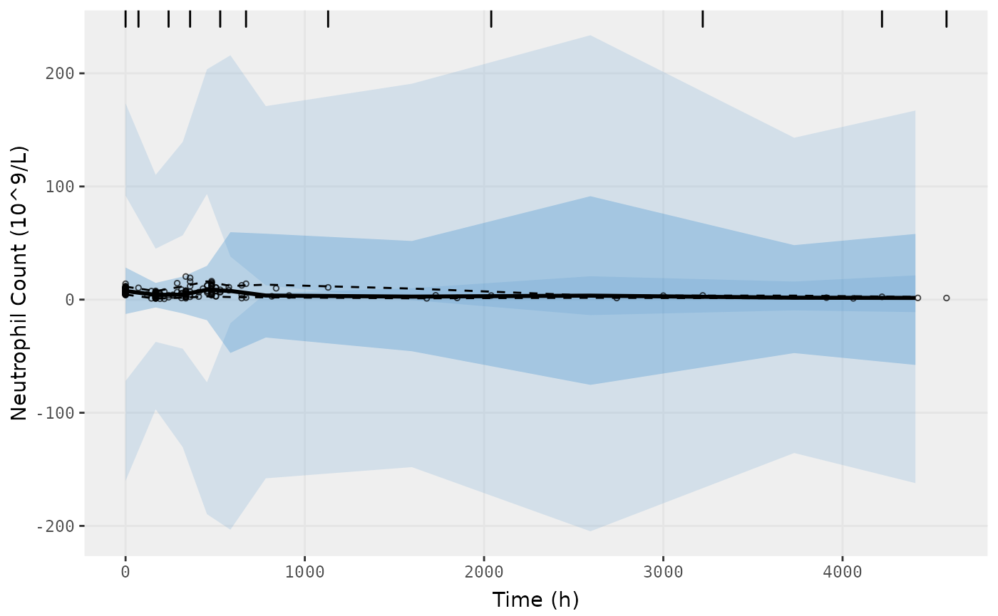


# specify bins
vpc.ui(fit.F, n=500, bins = c(0,170,300,350,500,600,900,3000,4580), show=list(obs_dv=T), ylab = "Neutrophil Count (10^9/L)", xlab = "Time (h)")
#> [====|====|====|====|====|====|====|====|====|====] 0:00:05
#>   $rxsim = original simulated data
#>   $sim = merge simulated data
#>   $obs = observed data
#>   $gg = vpc ggplot
#> use vpc(...) to change plot options
#> plotting the object now

Yuan Xiong

Fit model using saem

Fit model using FOCEi

FOCEi Goodness of fit plots