Example Model: Phenobarbitol with correlations

2022-03-26

nlmixr

Adding Covariances between random effects

You can simply add co-variances between two random effects by adding the effects together in the model specification block, that is eta.cl+eta.v ~. After that statement, you specify the lower triangular matrix of the fit with c().

An example of this is the phenobarbitol data:

## Load phenobarbitol data
library(nlmixr)

Model Specification

pheno <- function() {
  ini({
    tcl <- log(0.008) # typical value of clearance
    tv <-  log(0.6)   # typical value of volume
    ## var(eta.cl)
    eta.cl + eta.v ~ c(1, 
                       0.01, 1) ## cov(eta.cl, eta.v), var(eta.v)
                      # interindividual variability on clearance and volume
    add.err <- 0.1    # residual variability
  })
  model({
    cl <- exp(tcl + eta.cl) # individual value of clearance
    v <- exp(tv + eta.v)    # individual value of volume
    ke <- cl / v            # elimination rate constant
    d/dt(A1) = - ke * A1    # model differential equation
    cp = A1 / v             # concentration in plasma
    cp ~ add(add.err)       # define error model
  })
}

Fit with SAEM

fit <- nlmixr(pheno, pheno_sd, "saem",
              control=list(print=0), 
              table=list(cwres=TRUE, npde=TRUE))
#> [====|====|====|====|====|====|====|====|====|====] 0:00:00 
#> 
#> [====|====|====|====|====|====|====|====|====|====] 0:00:00 
#> 
#> [====|====|====|====|====|====|====|====|====|====] 0:00:00 
#> 
#> [====|====|====|====|====|====|====|====|====|====] 0:00:00 
#> 
#> [====|====|====|====|====|====|====|====|====|====] 0:00:00 
#> 
#> [====|====|====|====|====|====|====|====|====|====] 0:00:00

print(fit)
#> ── nlmixr SAEM(ODE); OBJF by FOCEi approximation fit ───────────────────────────
#> 
#>           OBJF      AIC      BIC Log-likelihood Condition Number
#> FOCEi 689.2758 986.1467 1004.407      -487.0734         7.845486
#> 
#> ── Time (sec $time): ───────────────────────────────────────────────────────────
#> 
#>          saem    setup table cwres covariance    other
#> elapsed 7.828 3.108015 0.987 4.123      0.019 1.074985
#> 
#> ── Population Parameters ($parFixed or $parFixedDf): ───────────────────────────
#> 
#>                          Parameter  Est.    SE %RSE    Back-transformed(95%CI)
#> tcl     typical value of clearance -5.01 0.077 1.54 0.00666 (0.00573, 0.00775)
#> tv         typical value of volume 0.351 0.053 15.1          1.42 (1.28, 1.58)
#> add.err       residual variability  2.84                                  2.84
#>         BSV(CV%) Shrink(SD)%
#> tcl         54.7      1.78% 
#> tv          40.3      1.21% 
#> add.err                     
#>  
#>   Covariance Type ($covMethod): linFim
#>   Some strong fixed parameter correlations exist ($cor) :
#>     cor:tv,tcl 
#>     0.735  
#>  
#> 
#>   Correlations in between subject variability (BSV) matrix:
#>     cor:eta.v,eta.cl 
#>           0.987  
#>  
#> 
#>   Full BSV covariance ($omega) or correlation ($omegaR; diagonals=SDs) 
#>   Distribution stats (mean/skewness/kurtosis/p-value) available in $shrink 
#> 
#> ── Fit Data (object is a modified tibble): ─────────────────────────────────────
#> # A tibble: 155 × 24
#>   ID     TIME    DV EPRED  ERES   NPDE    NPD  PRED    RES    WRES IPRED  IRES
#>   <fct> <dbl> <dbl> <dbl> <dbl>  <dbl>  <dbl> <dbl>  <dbl>   <dbl> <dbl> <dbl>
#> 1 1        2   17.3  18.7 -1.43 -0.403 -0.403  17.4 -0.132 -0.0180  18.4 -1.07
#> 2 1      112.  31    29.9  1.08  0.376  0.376  27.9  3.05   0.248   29.7  1.33
#> 3 2        2    9.7  10.8 -1.12 -1.01  -1.01   10.5 -0.759 -0.153   12.4 -2.65
#> # … with 152 more rows, and 12 more variables: IWRES <dbl>, CPRED <dbl>,
#> #   CRES <dbl>, CWRES <dbl>, eta.cl <dbl>, eta.v <dbl>, A1 <dbl>, cl <dbl>,
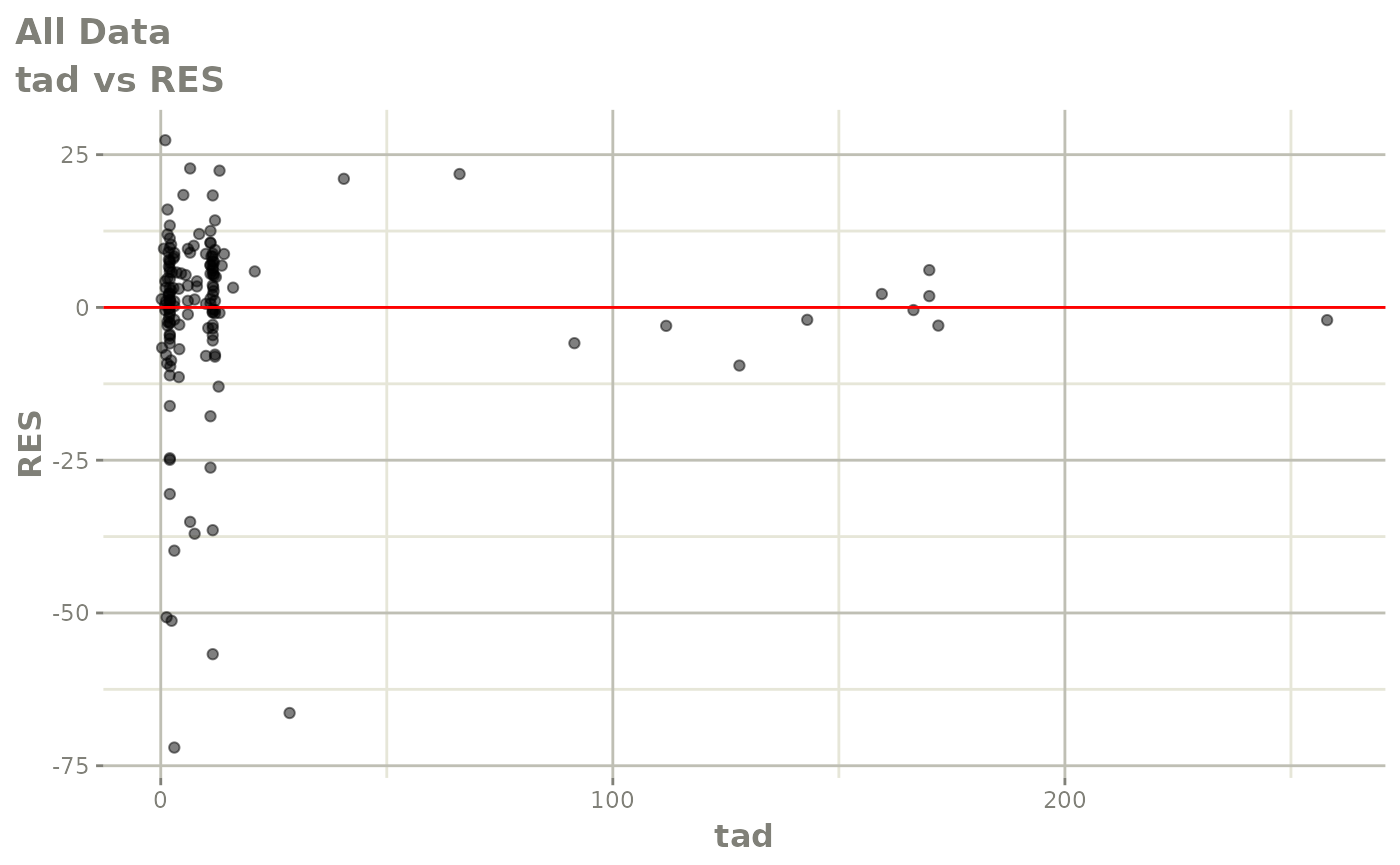
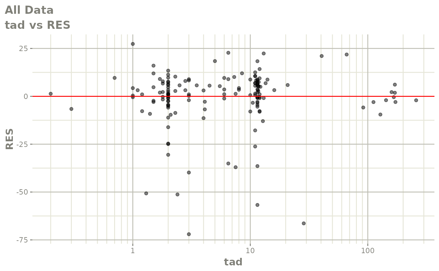
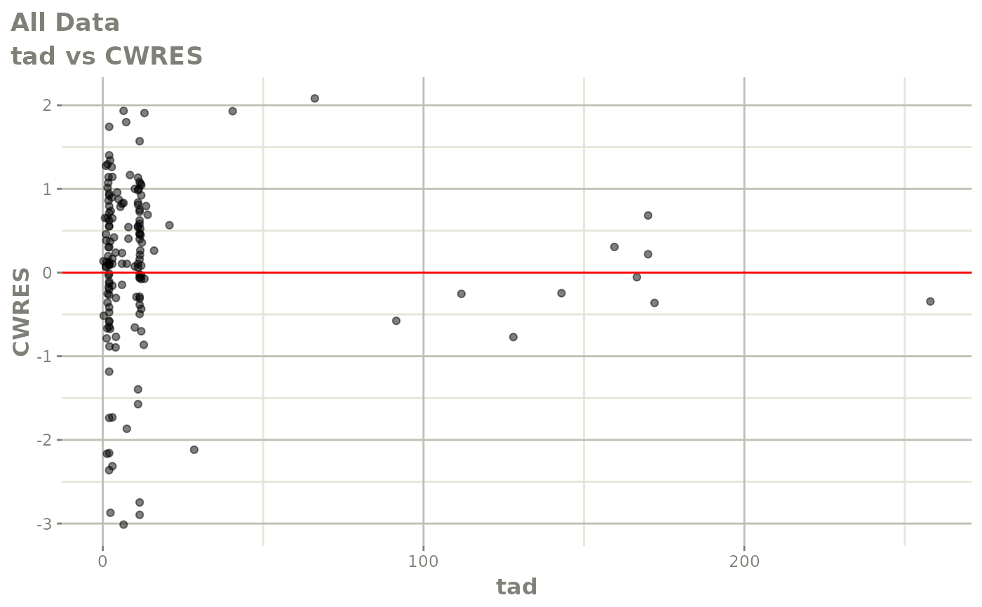
#> #   v <dbl>, ke <dbl>, tad <dbl>, dosenum <dbl>

Basic Goodness of Fit Plots

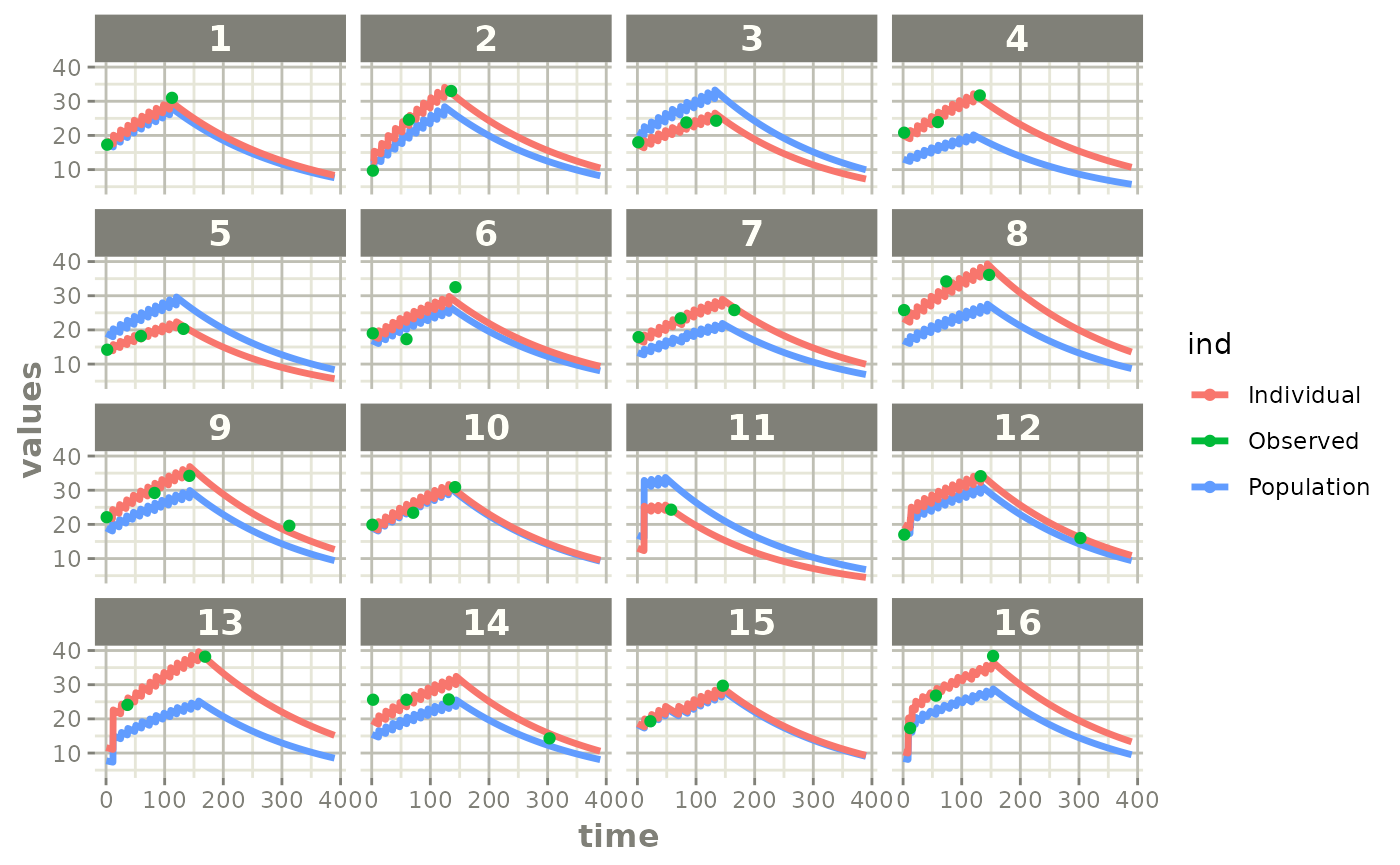
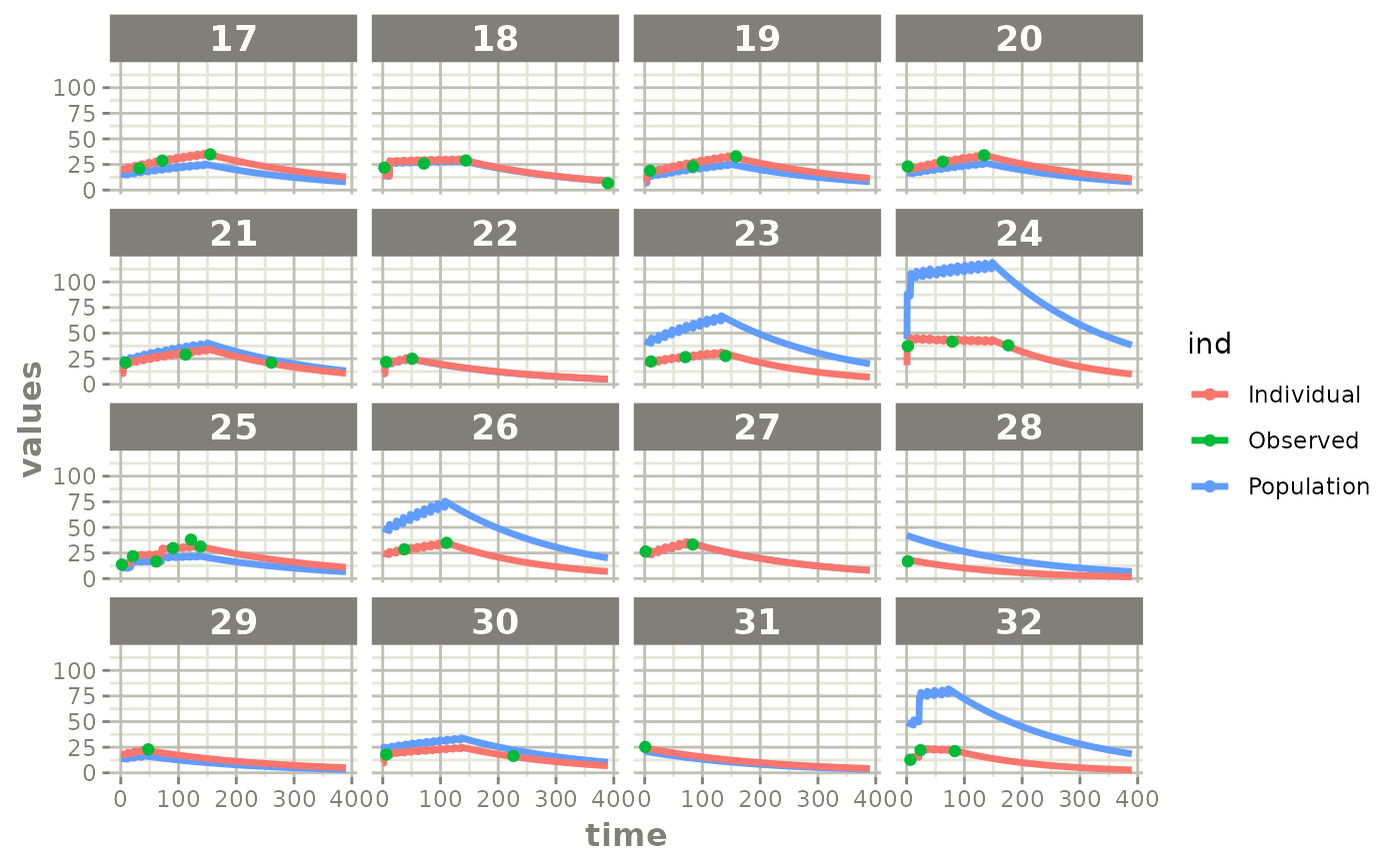
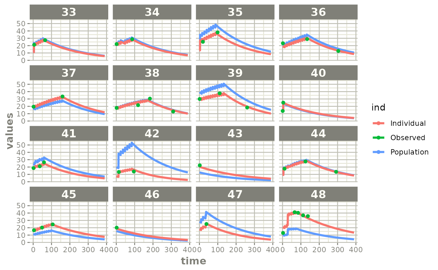
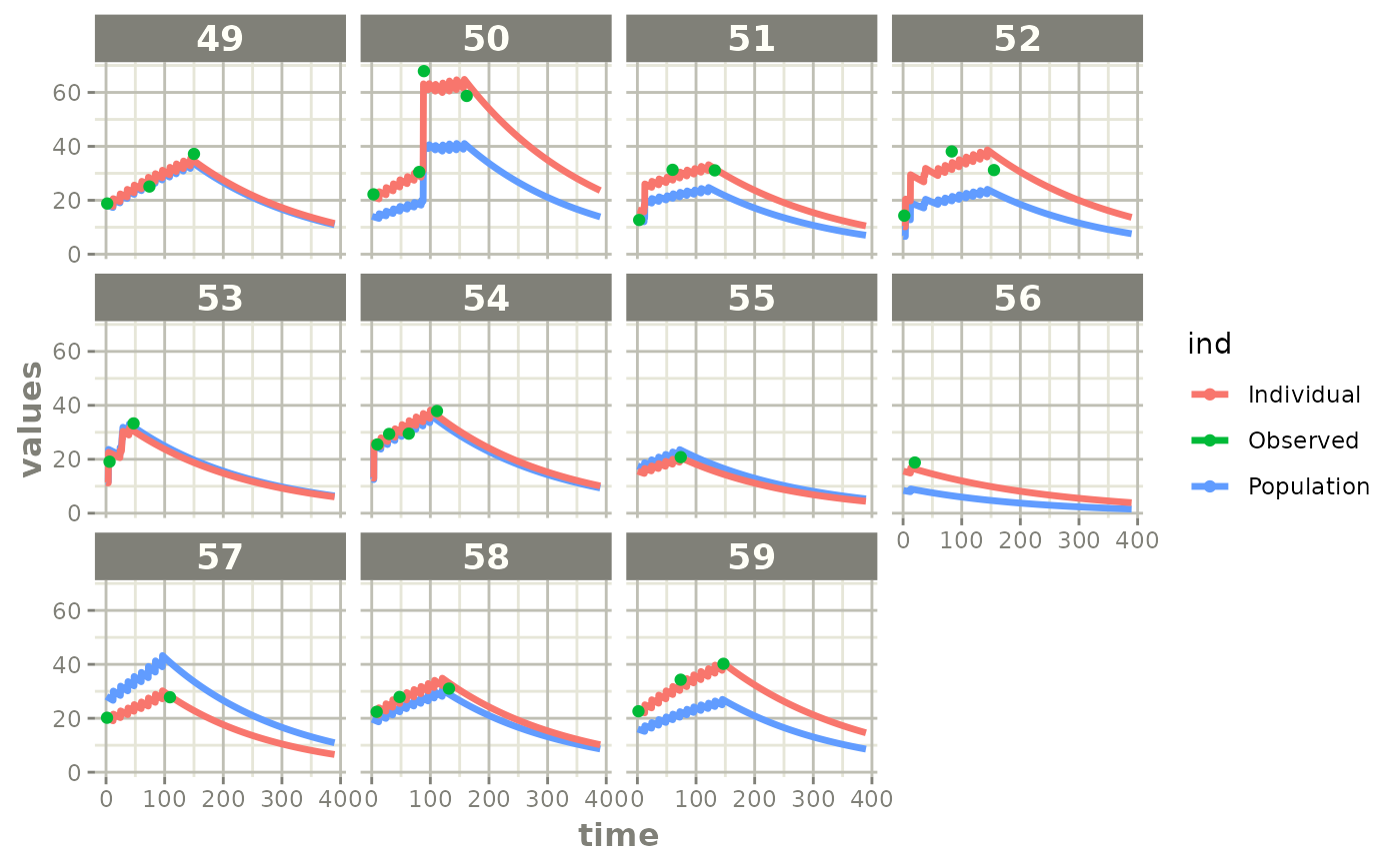
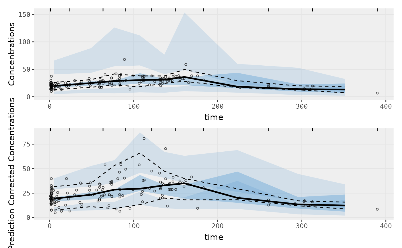
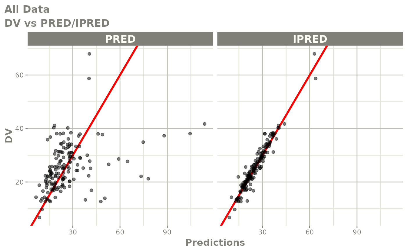
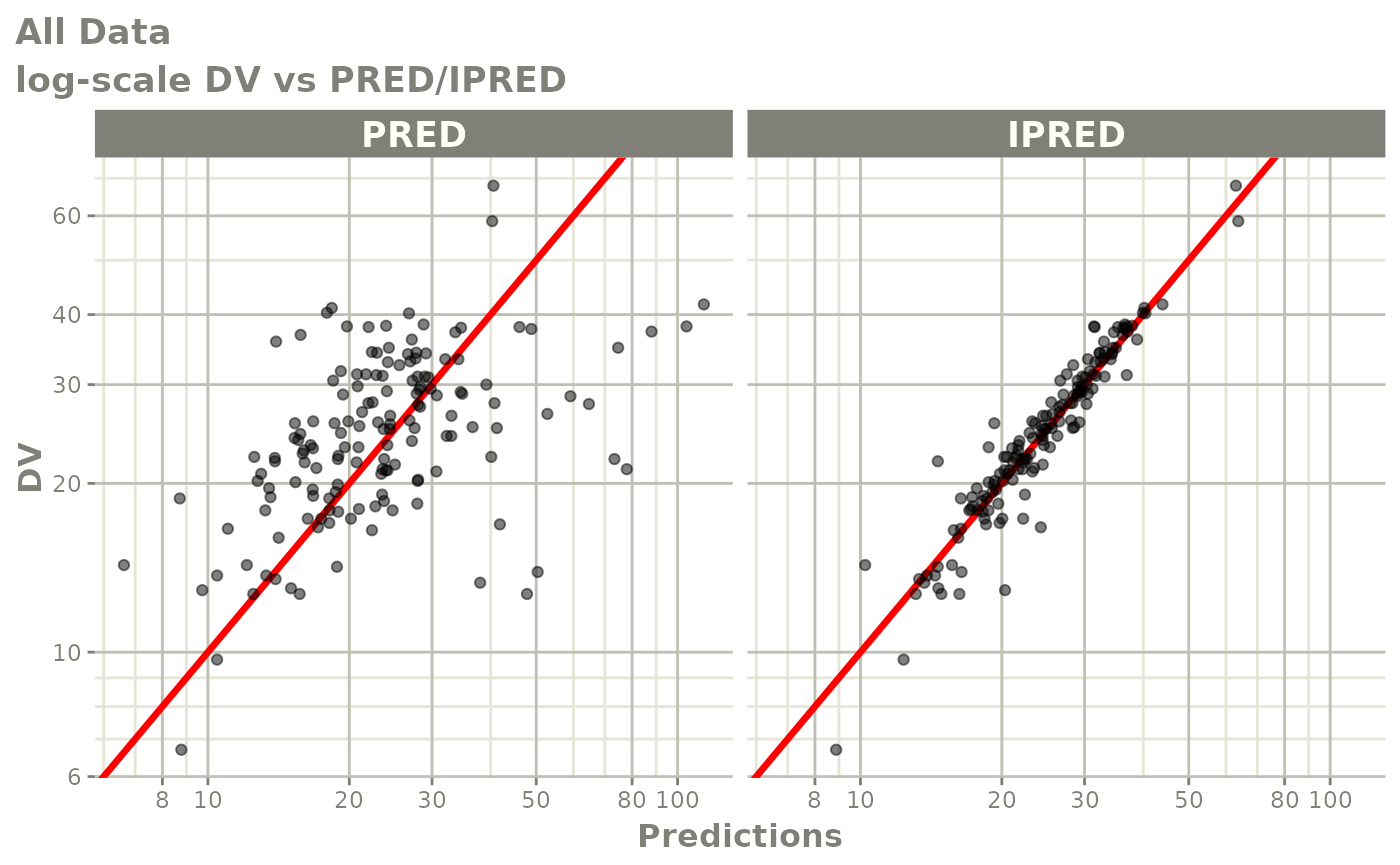
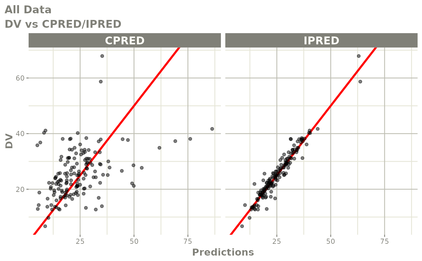
plot(fit)

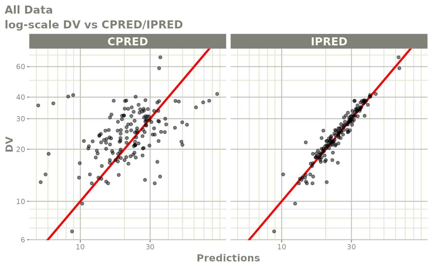
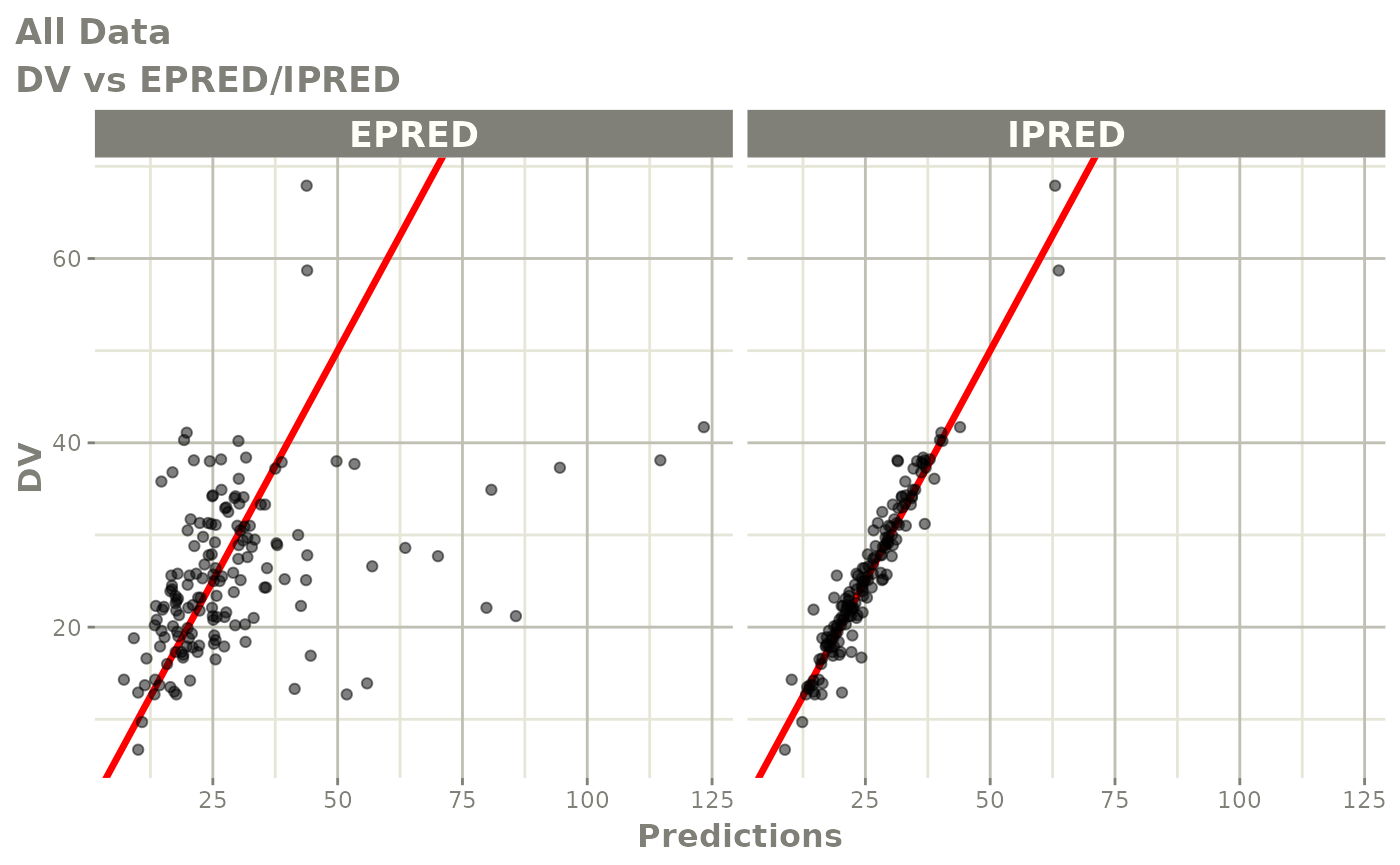
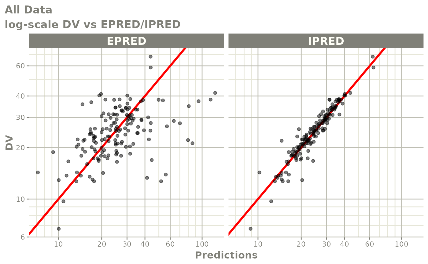
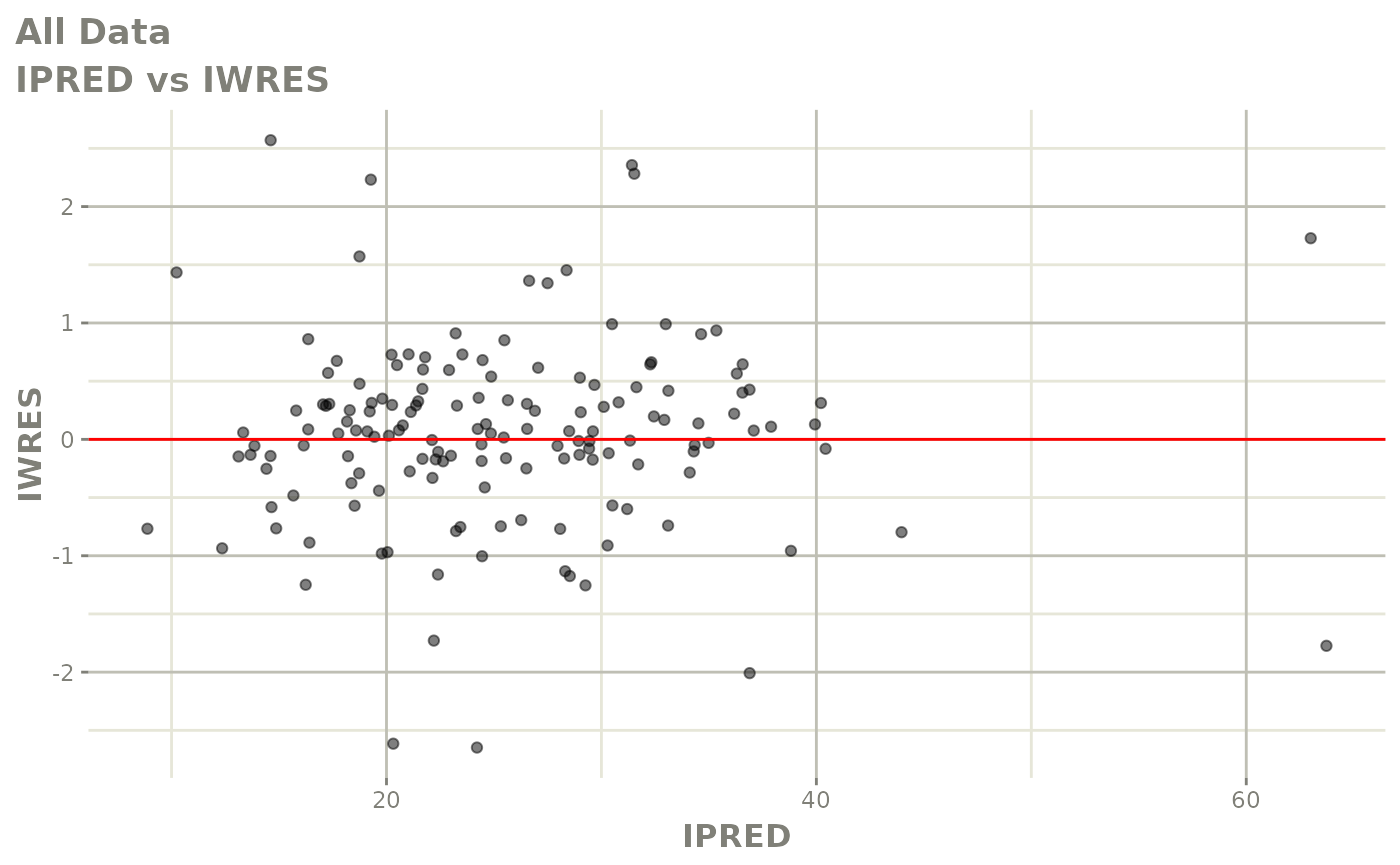
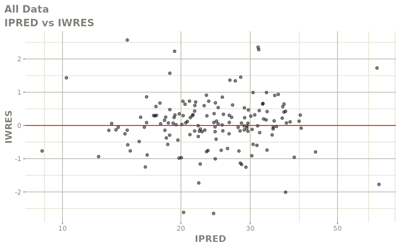
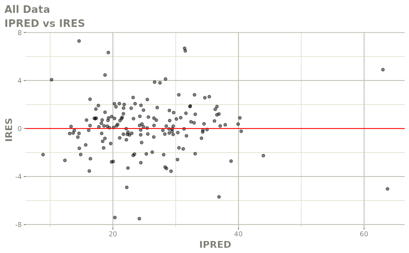
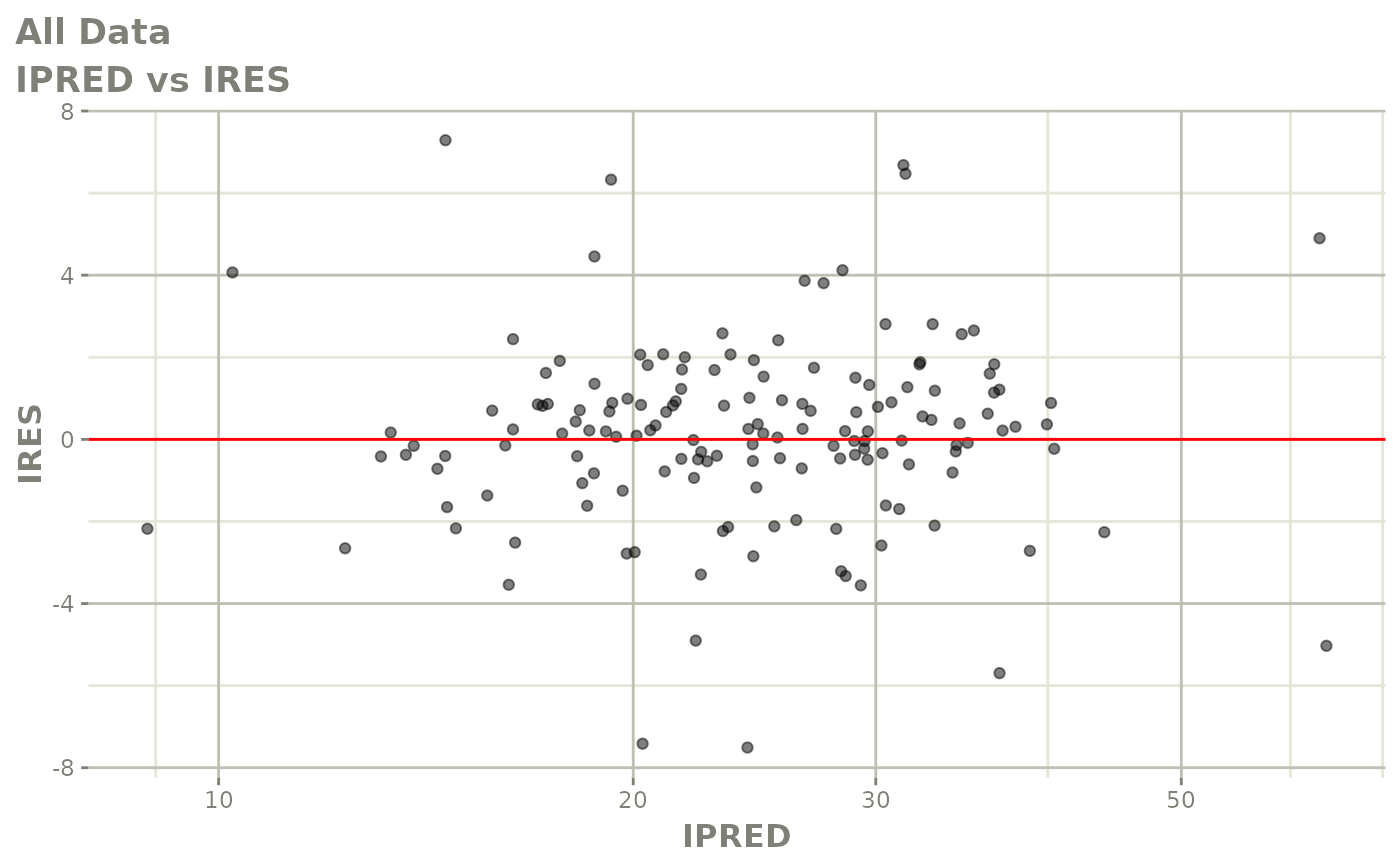
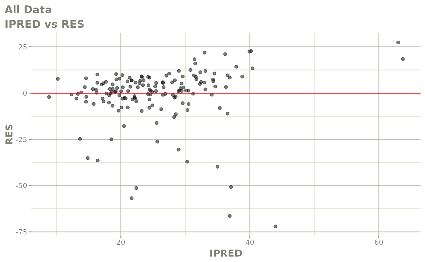
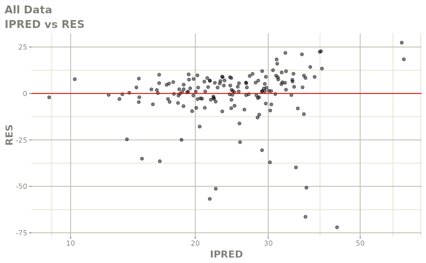
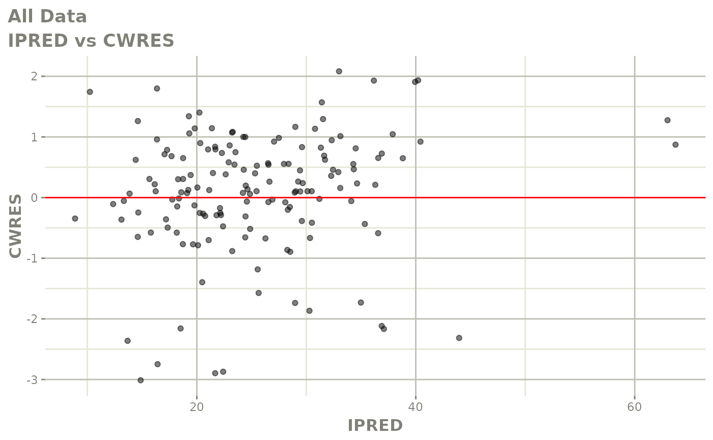
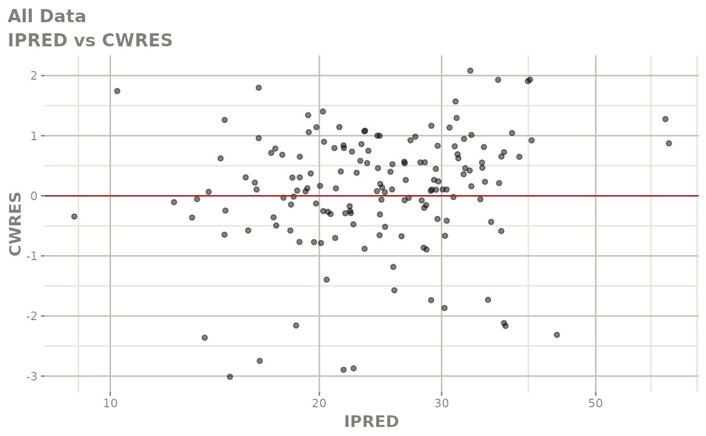
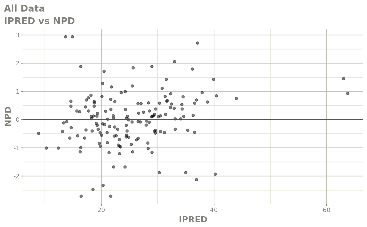
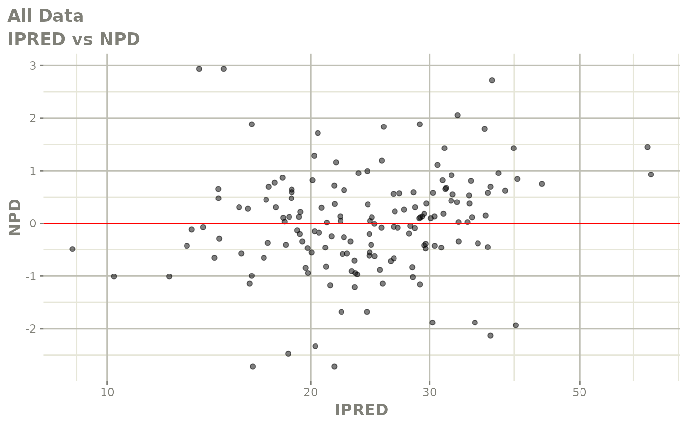
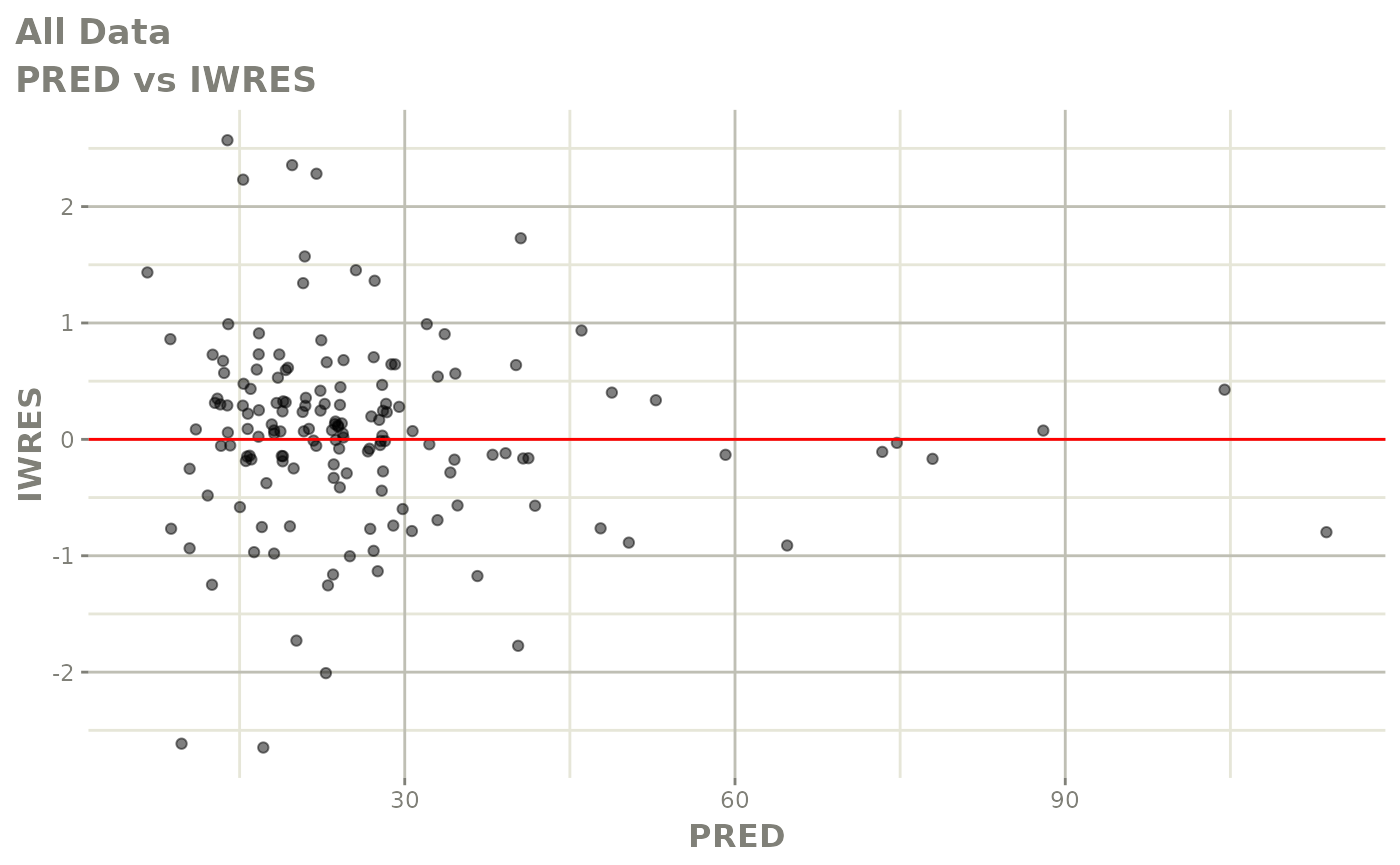
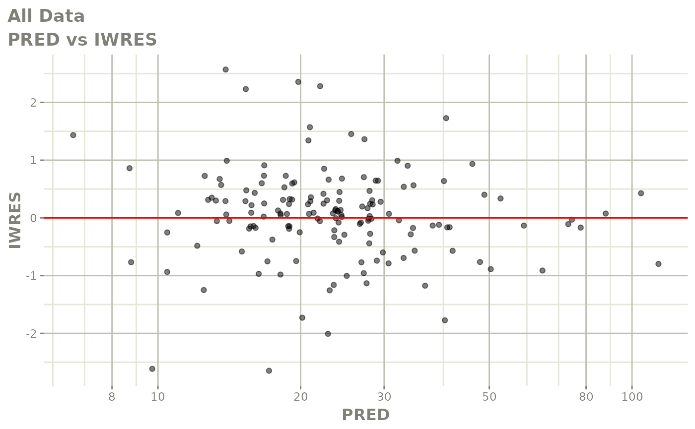
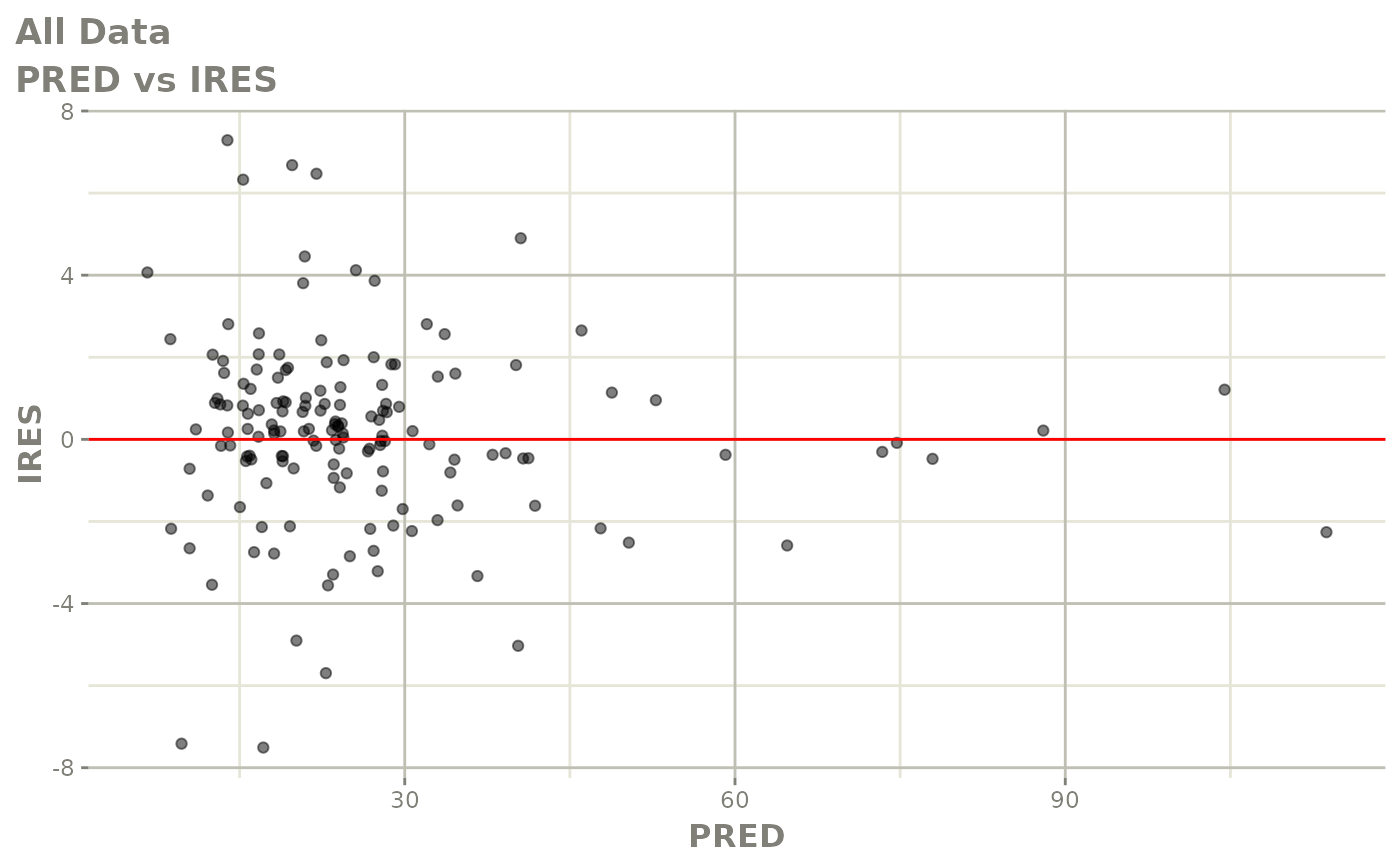
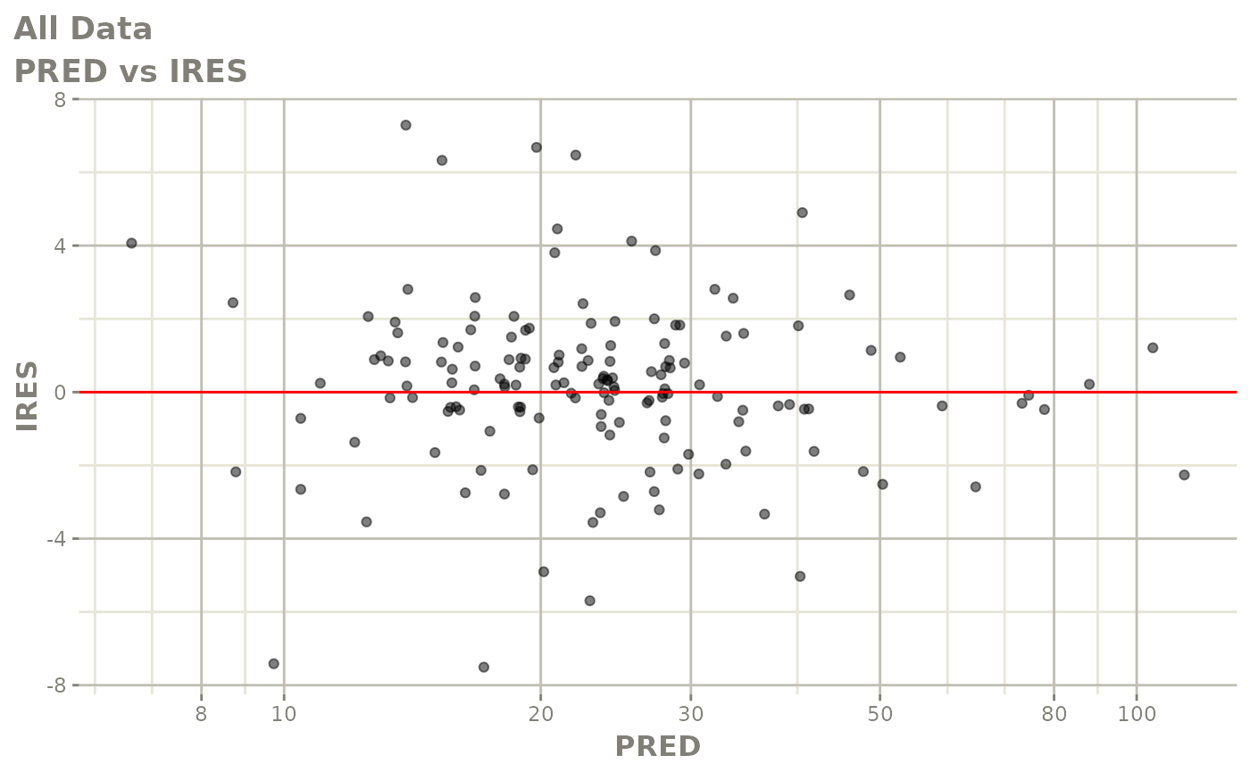
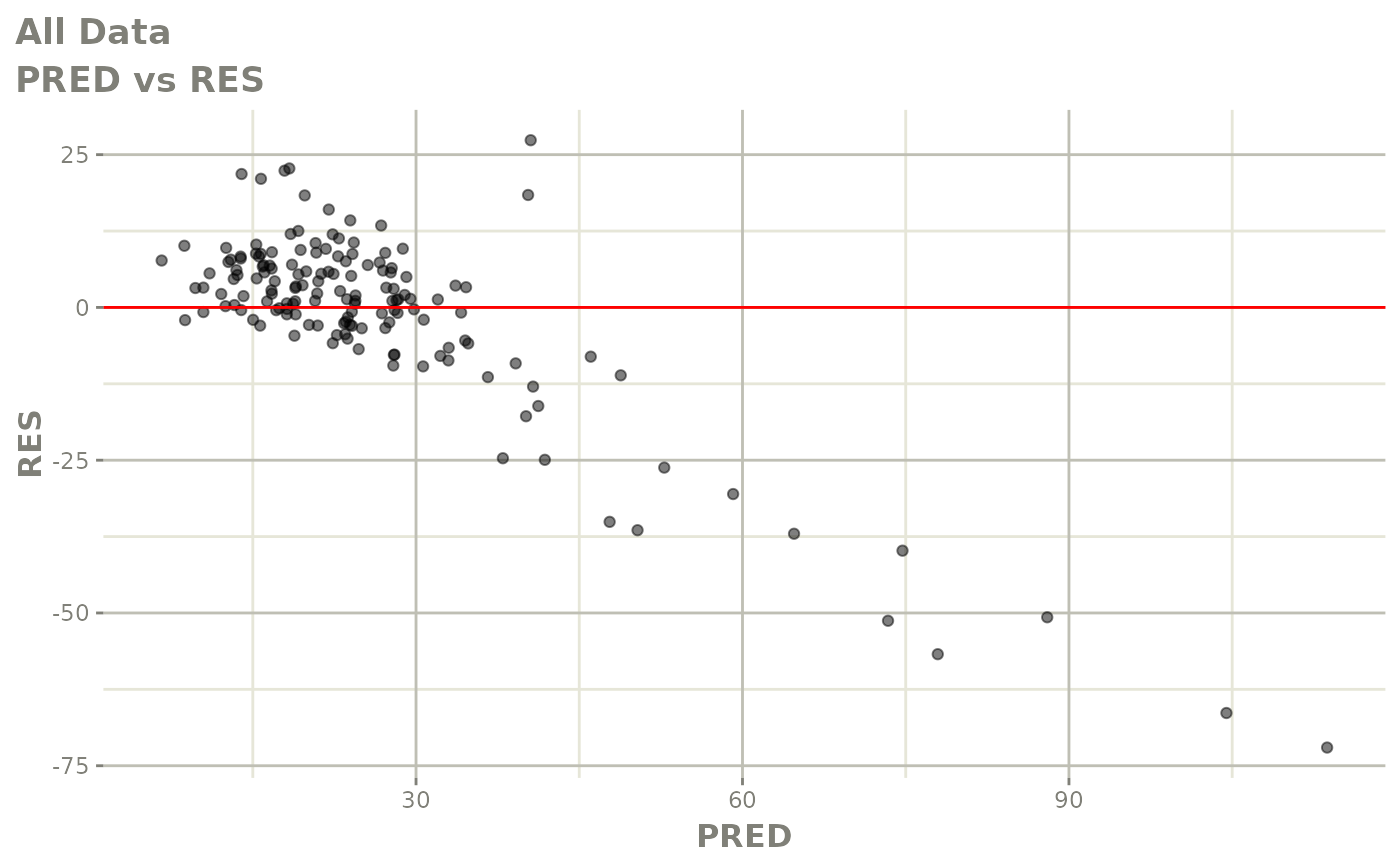
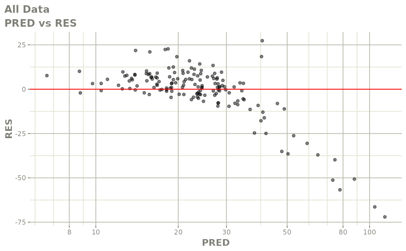
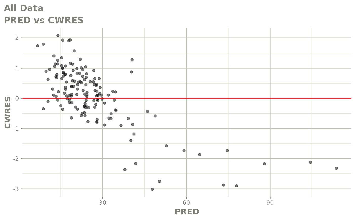
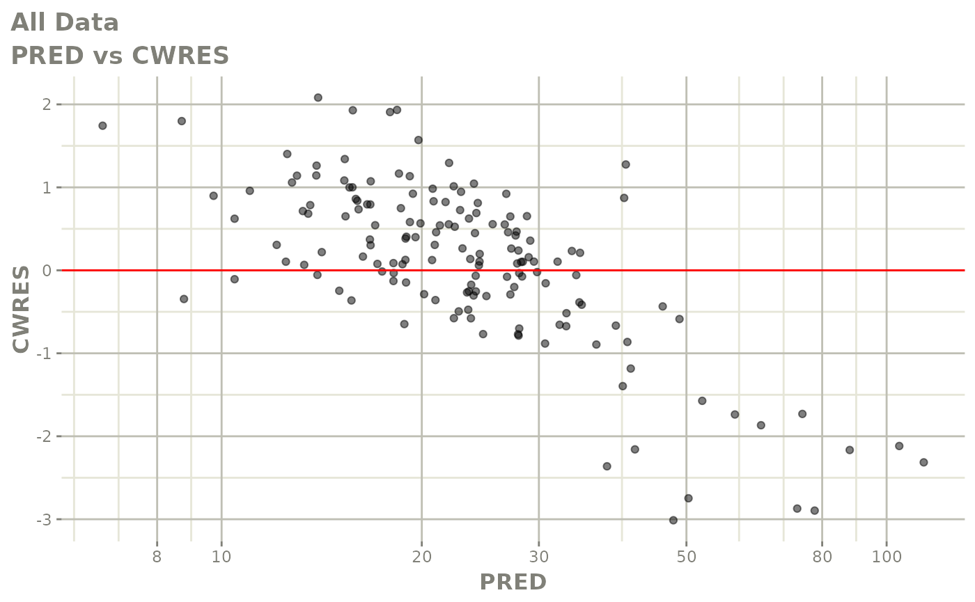
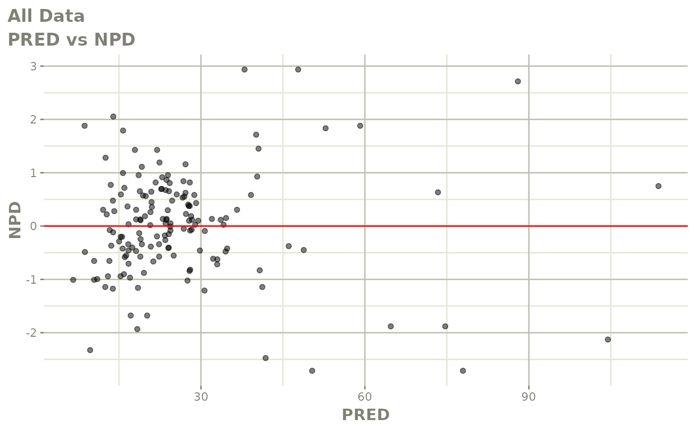
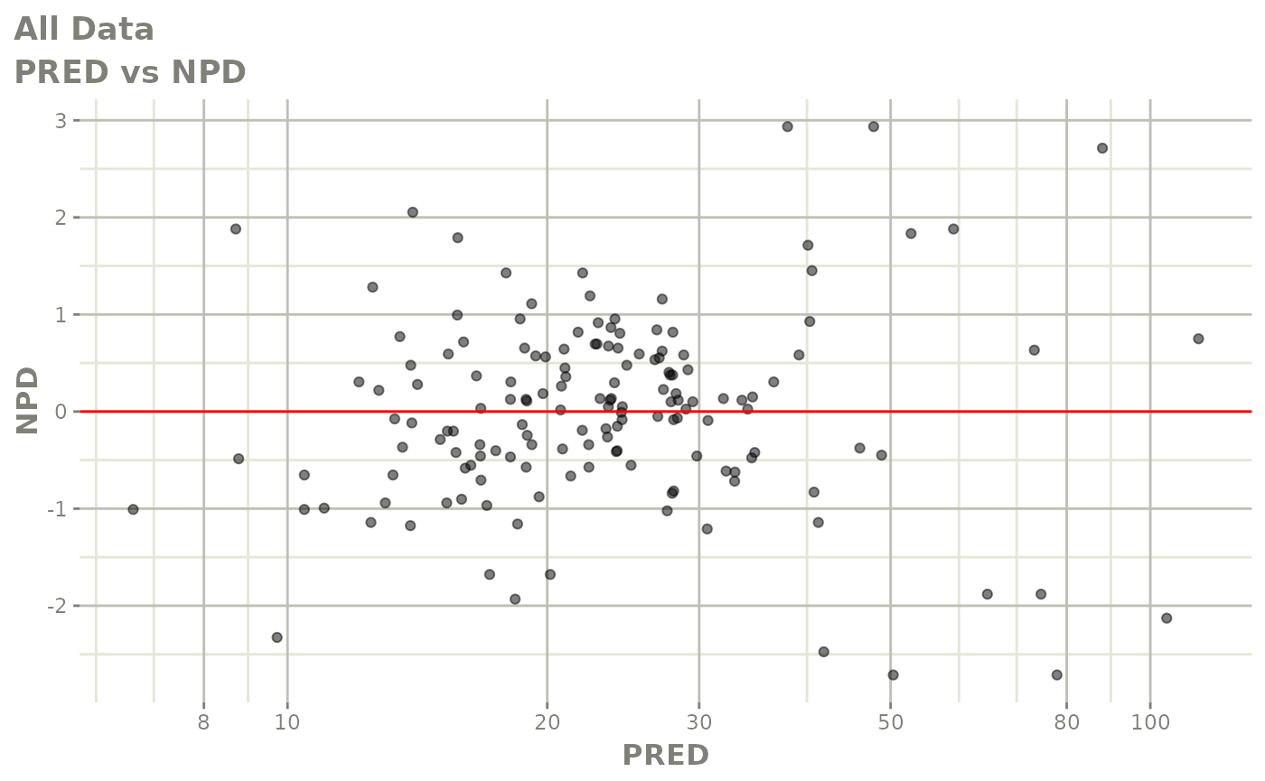
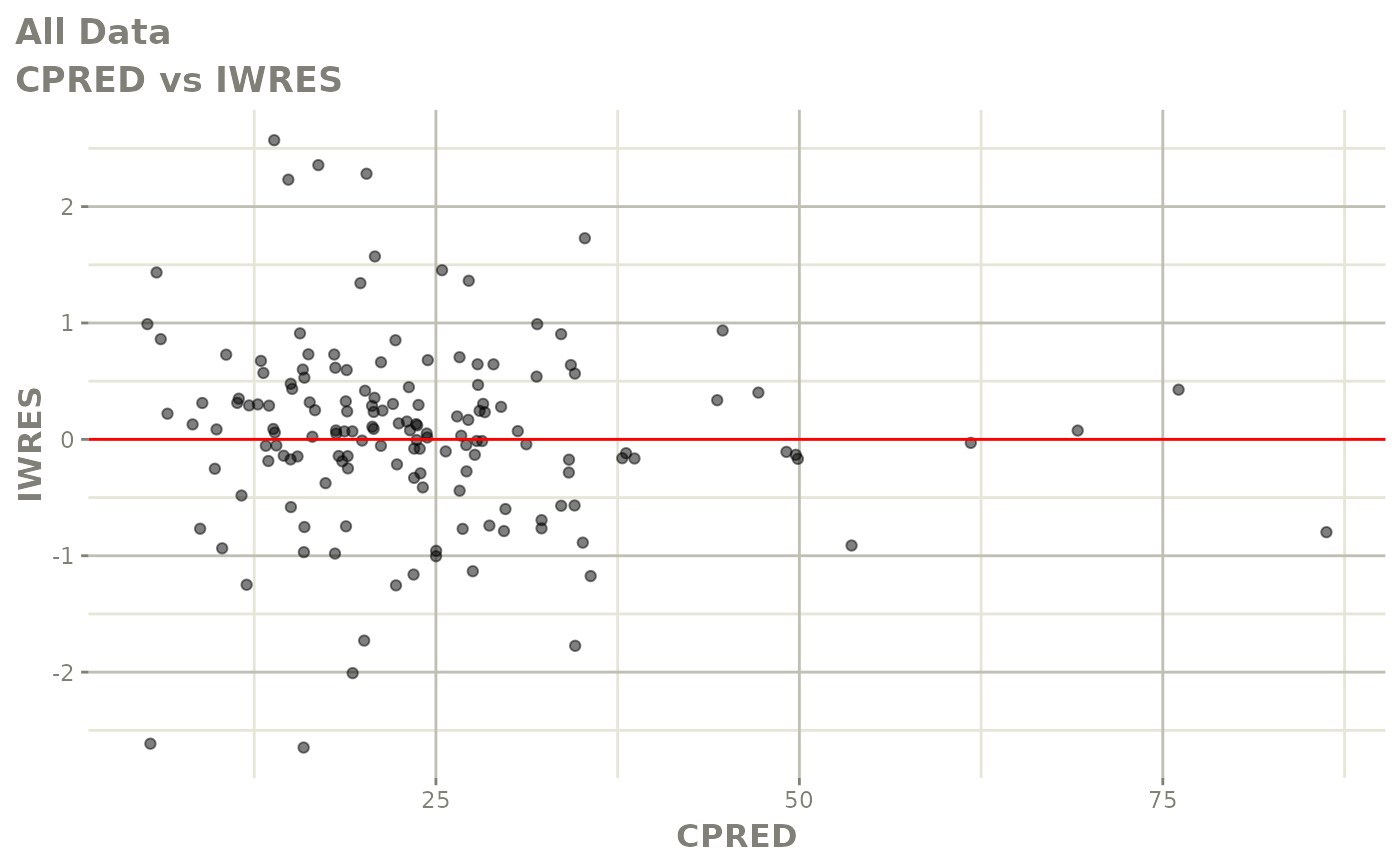
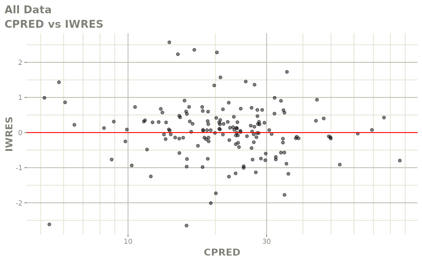
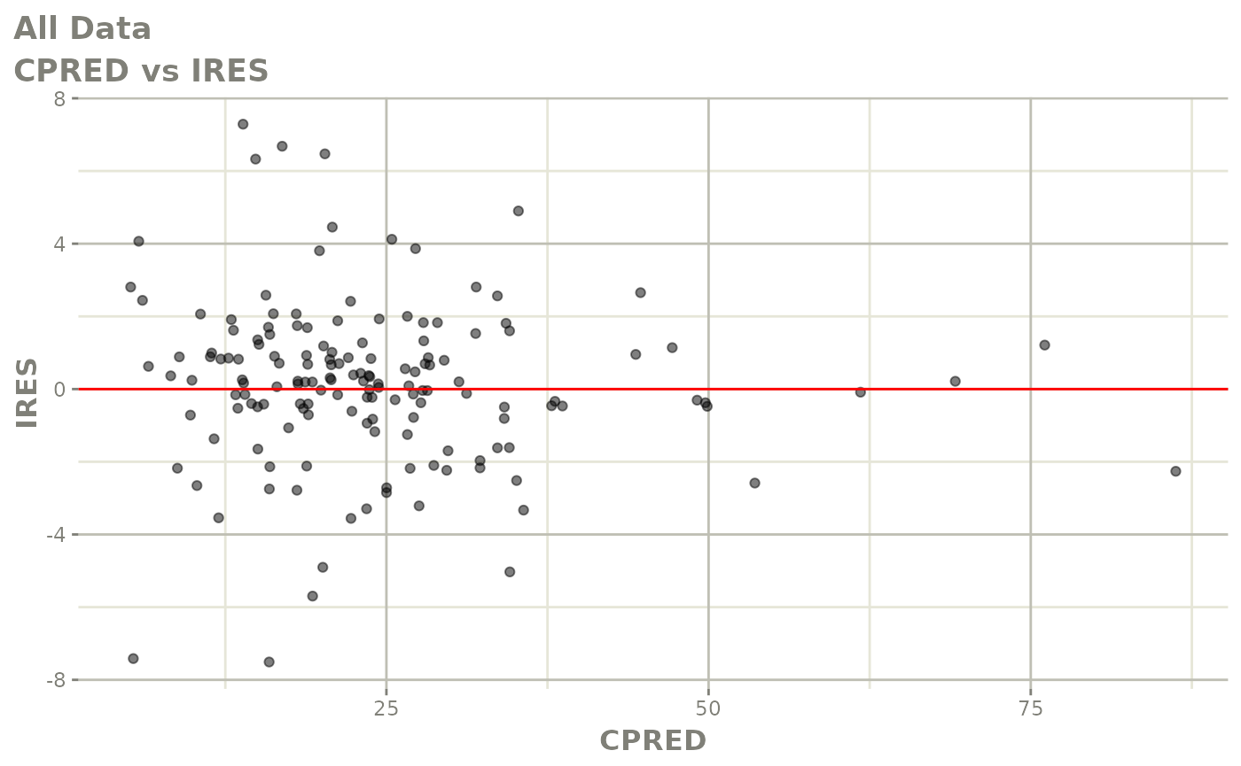
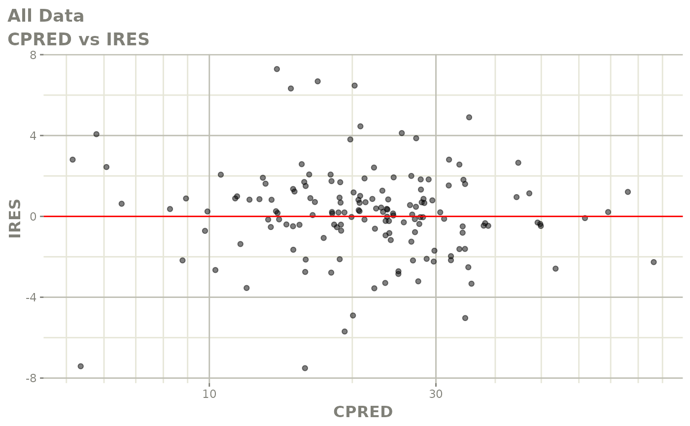
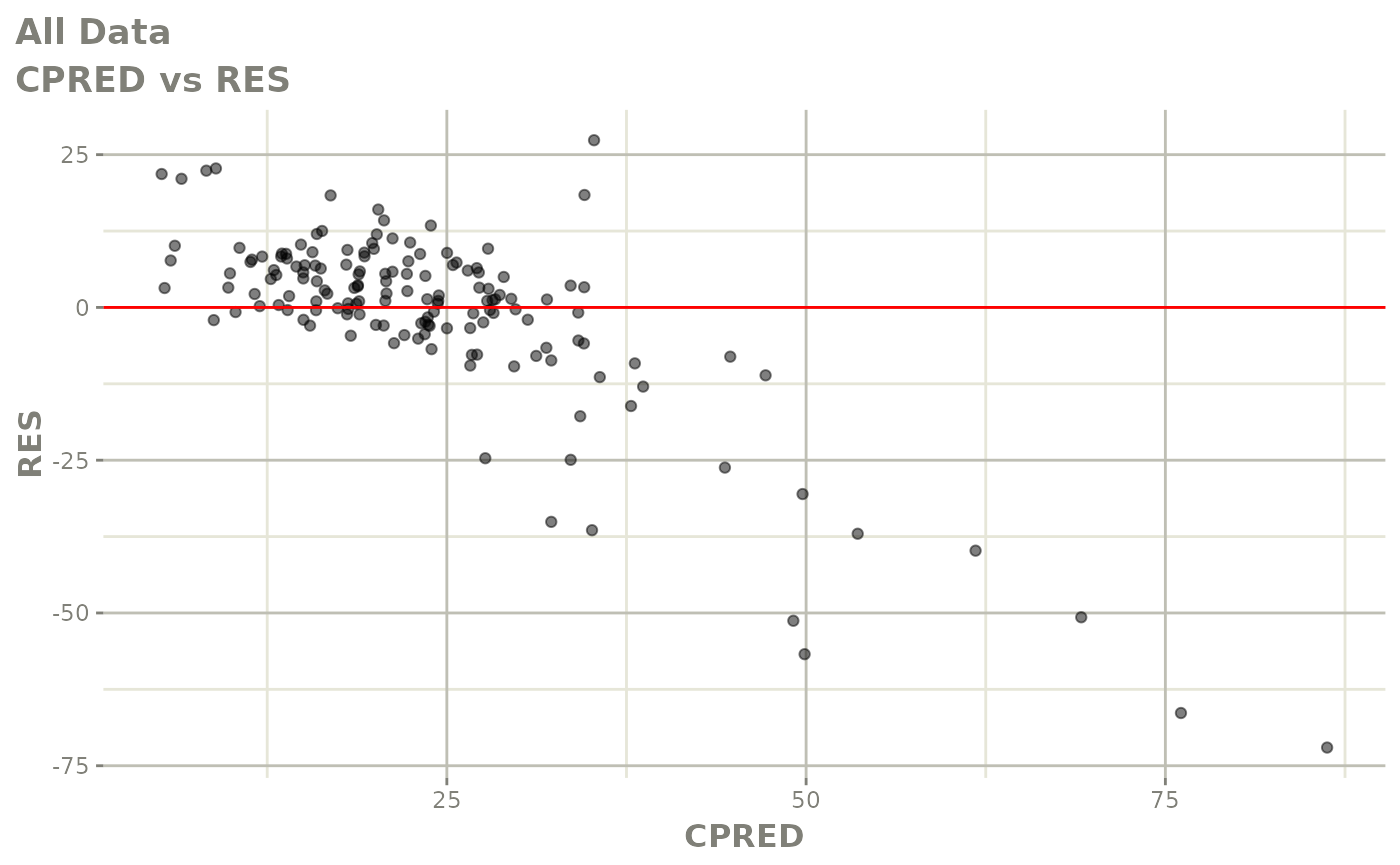
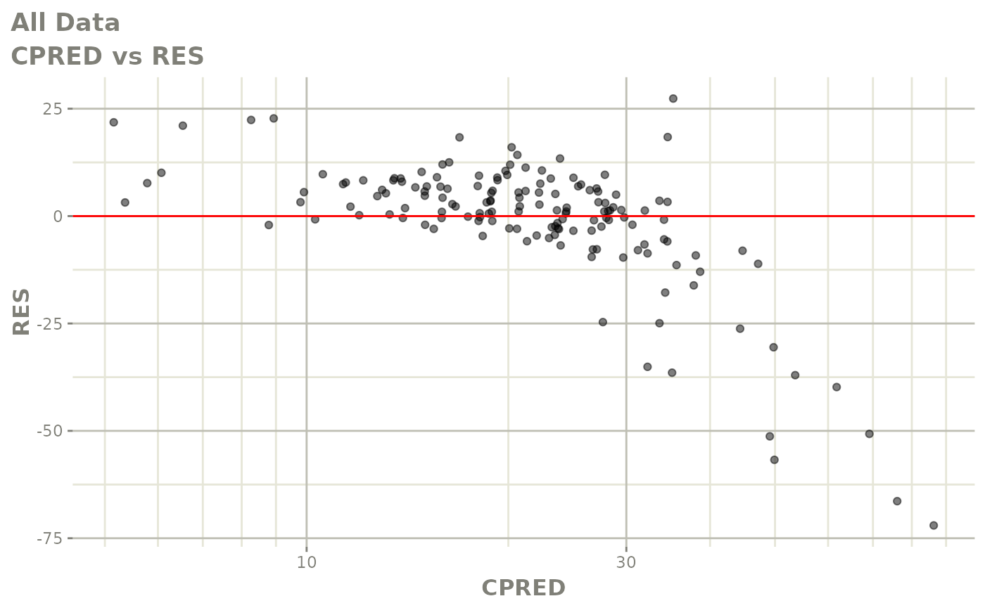
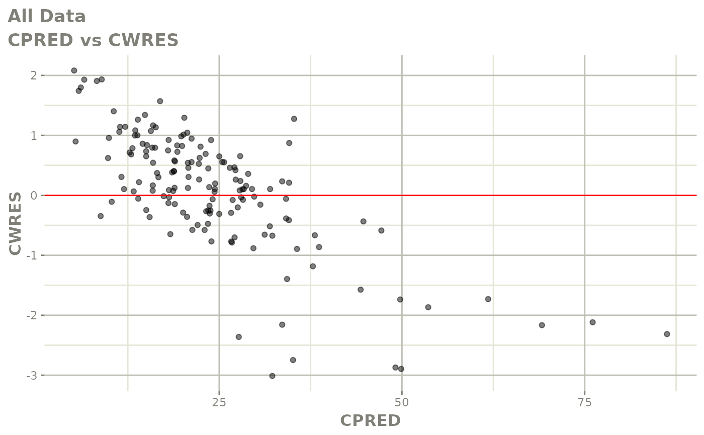
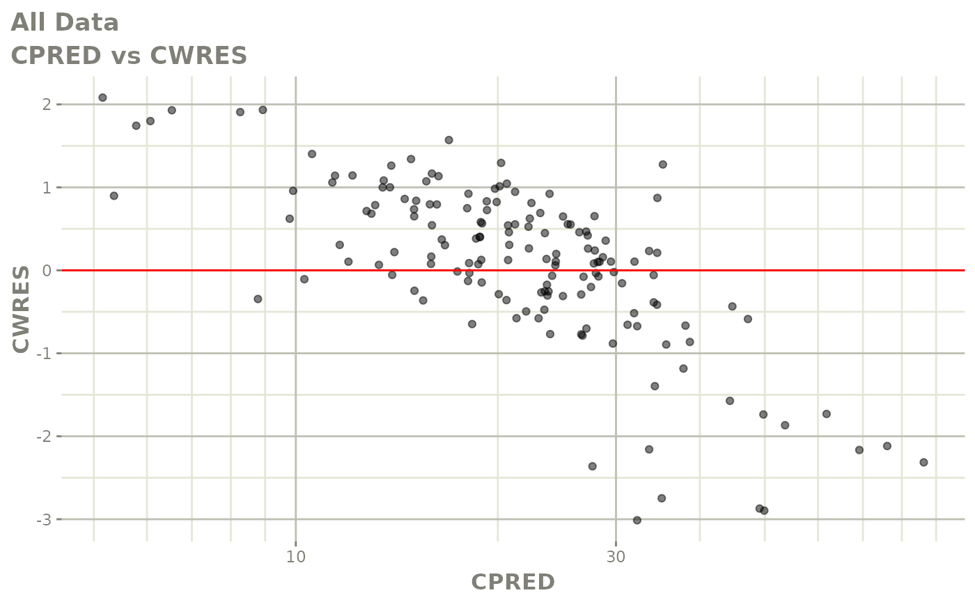
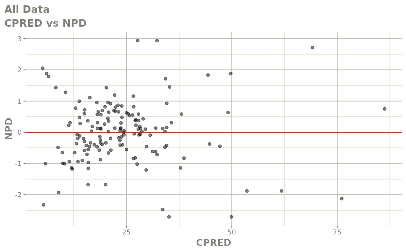
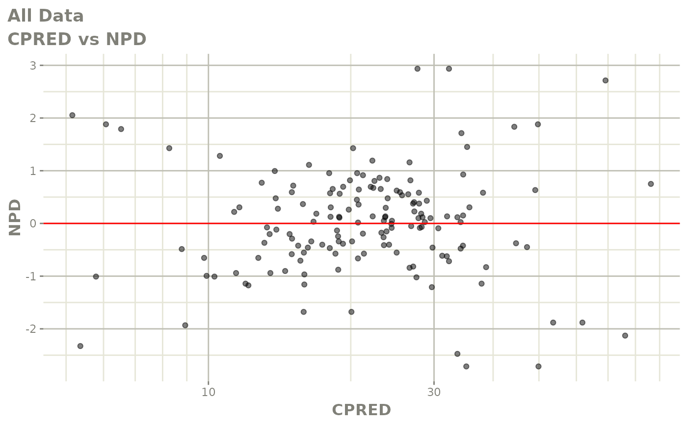
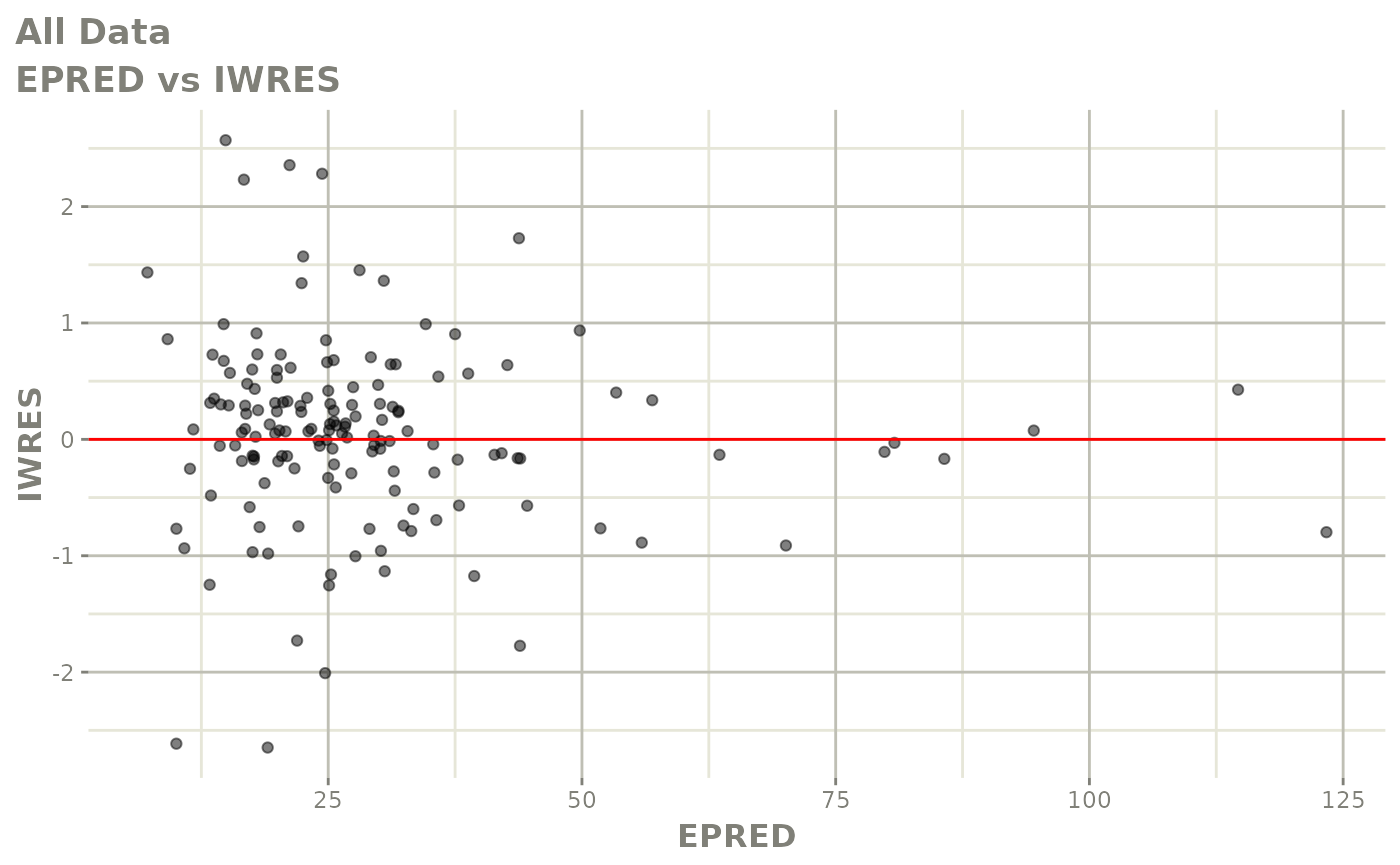
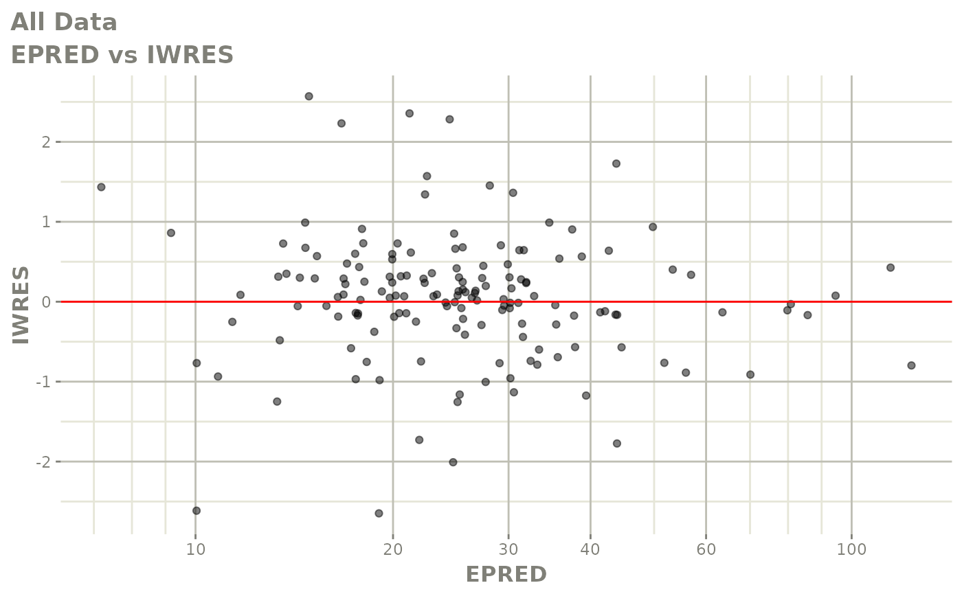
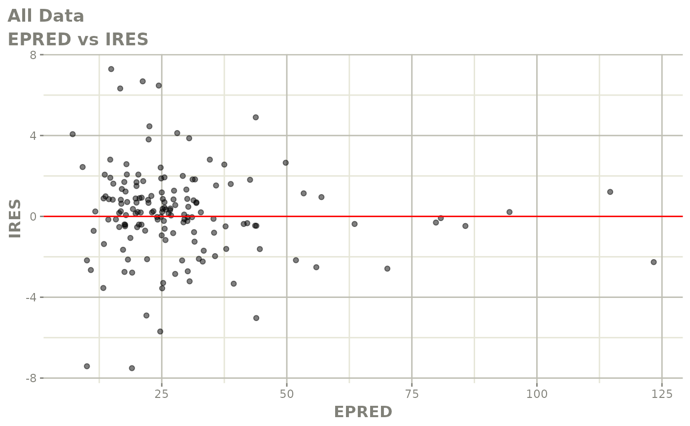
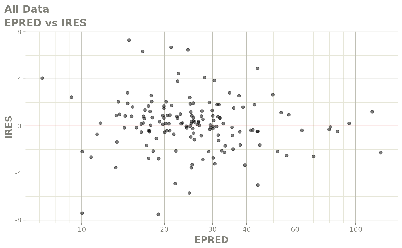
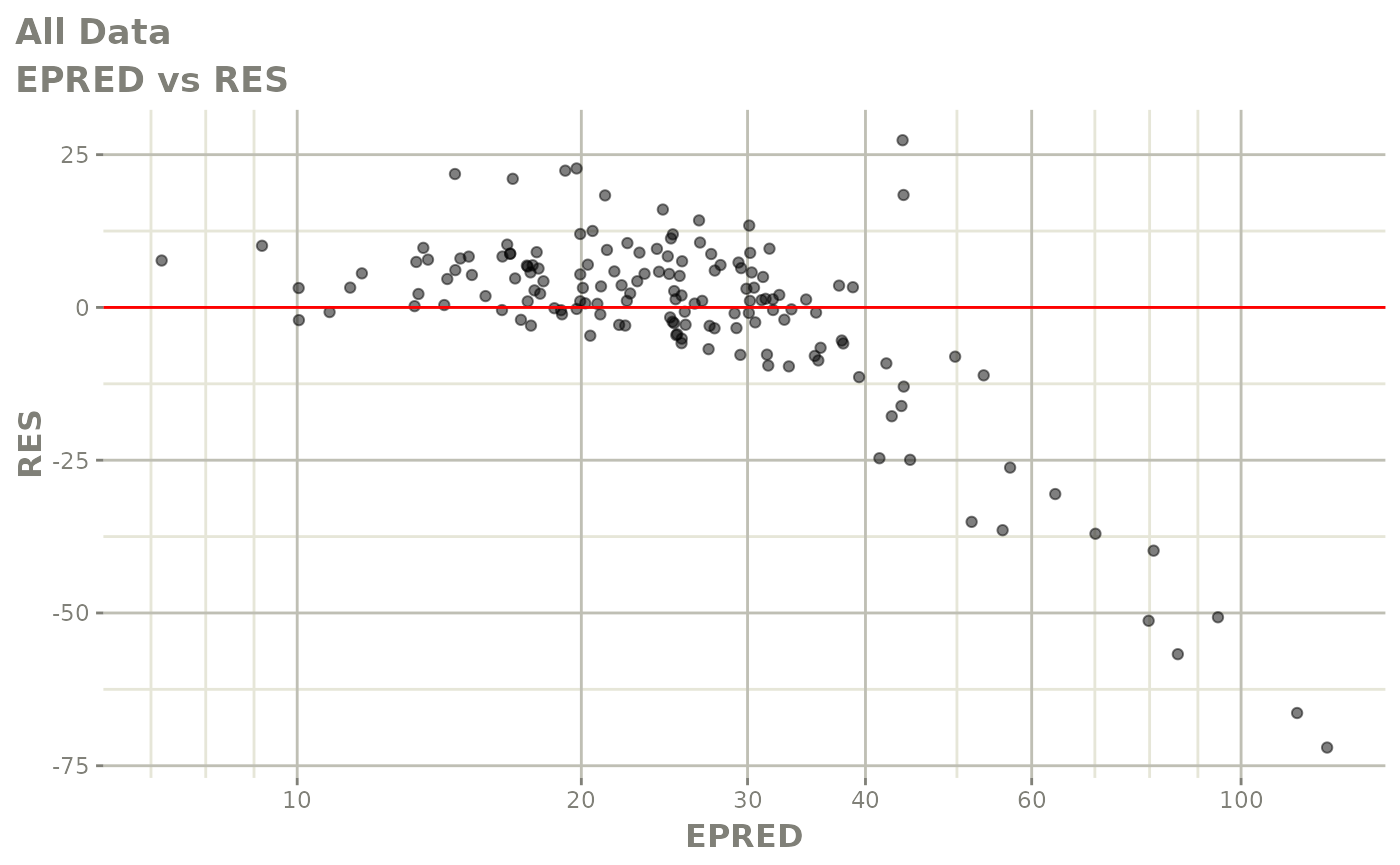
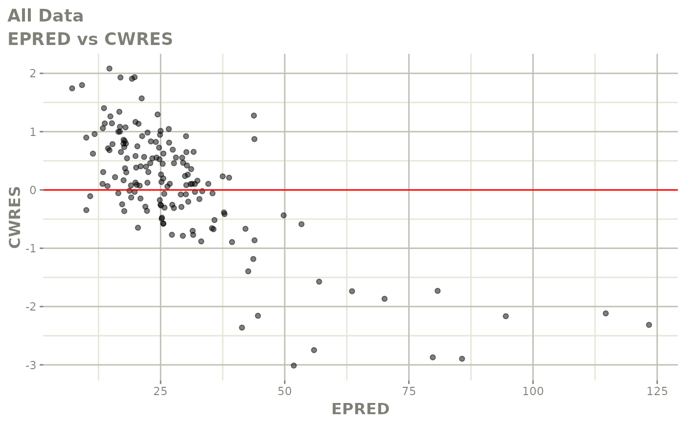
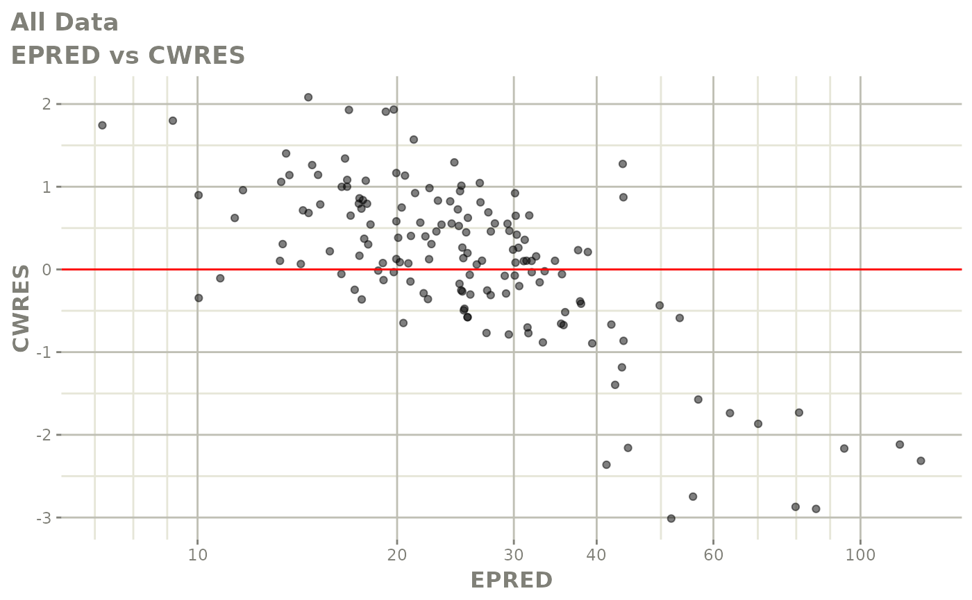
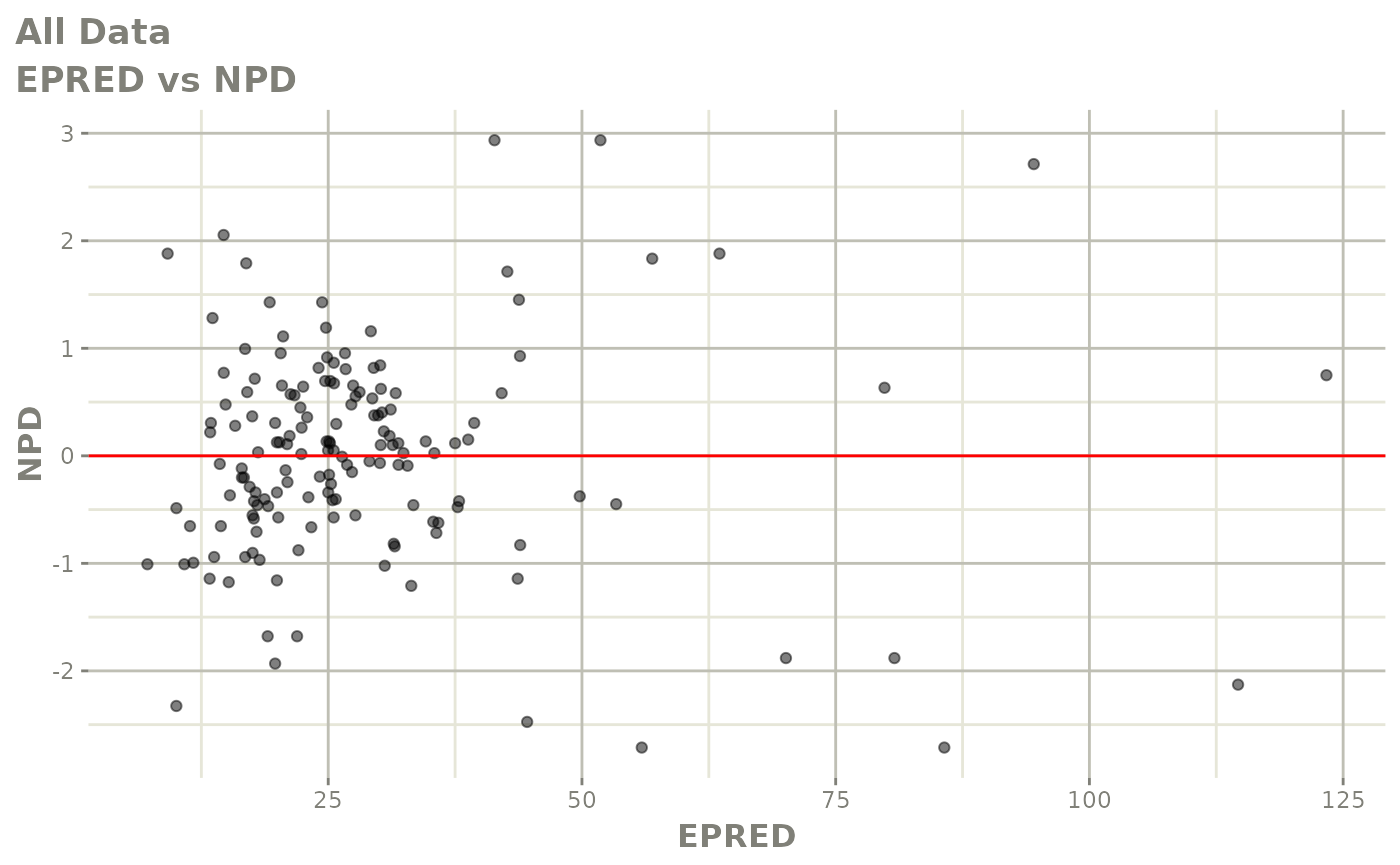
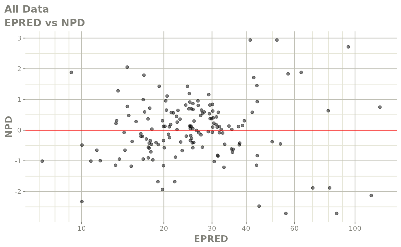
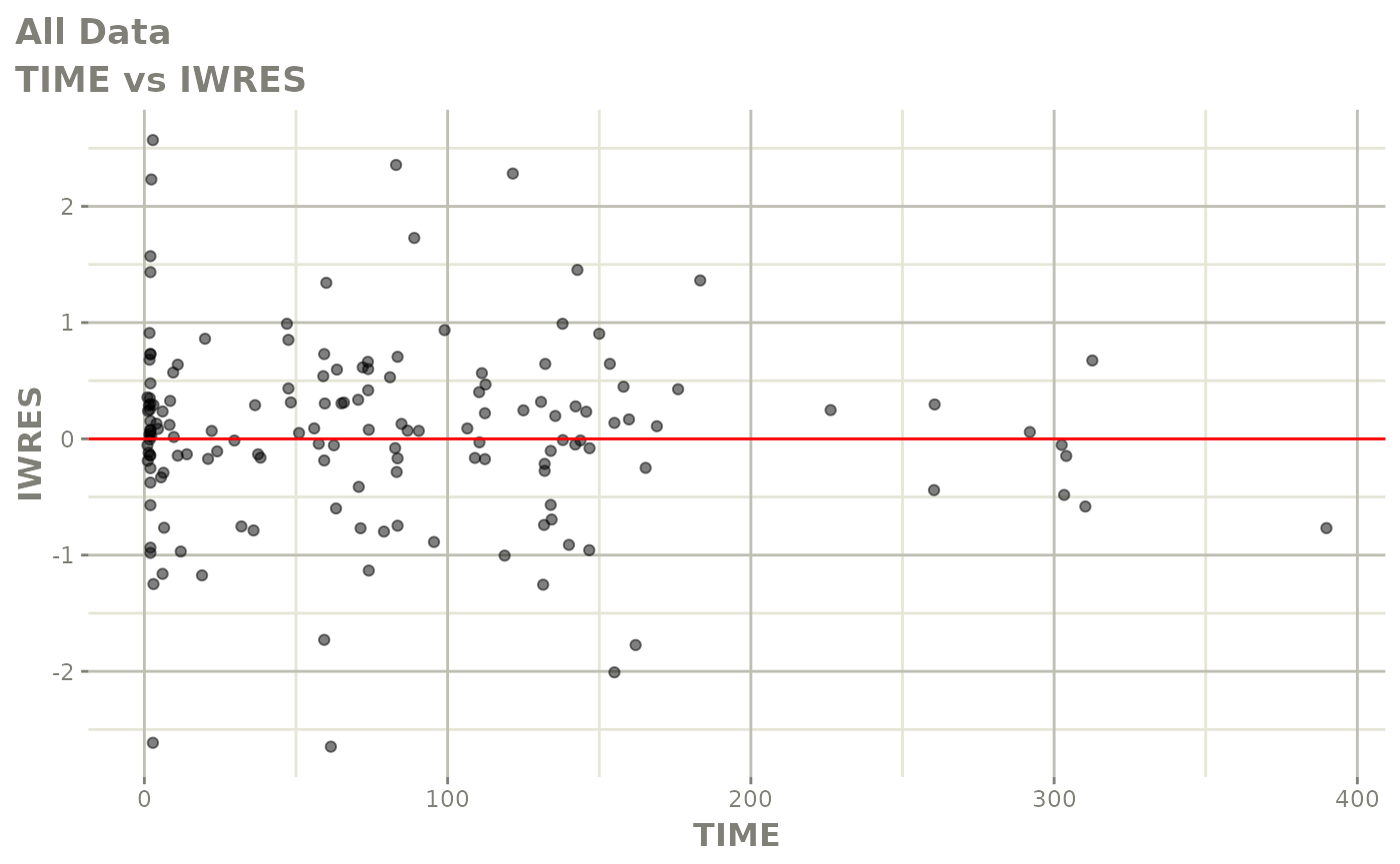
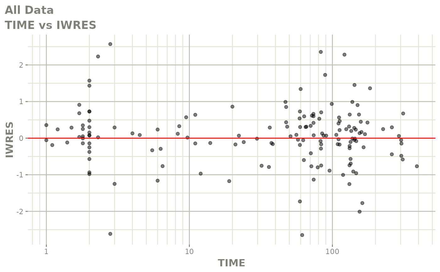
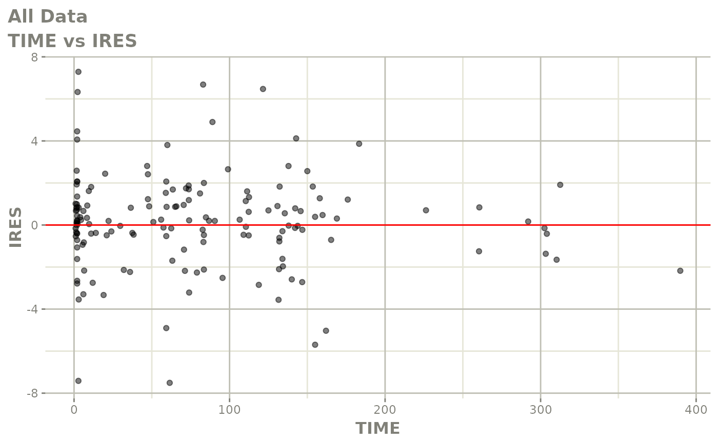
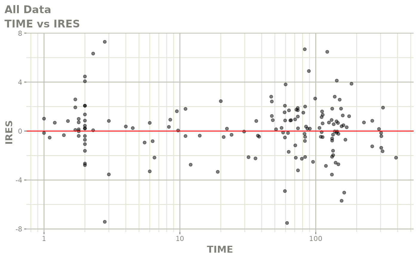
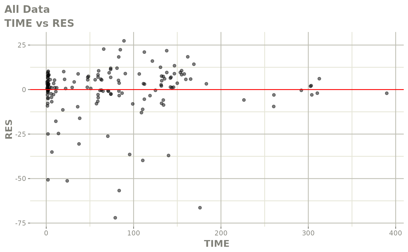
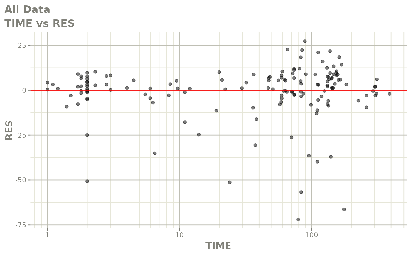
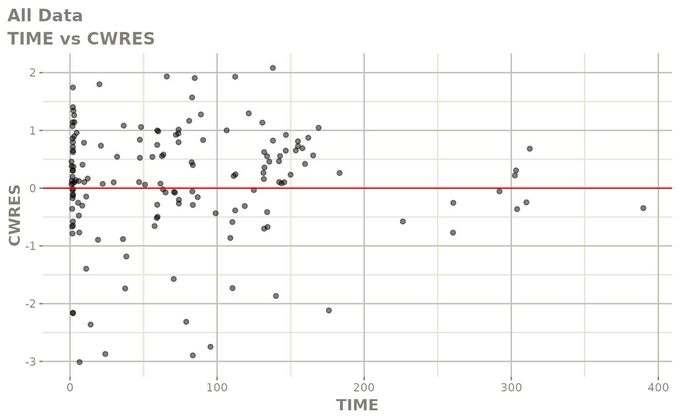
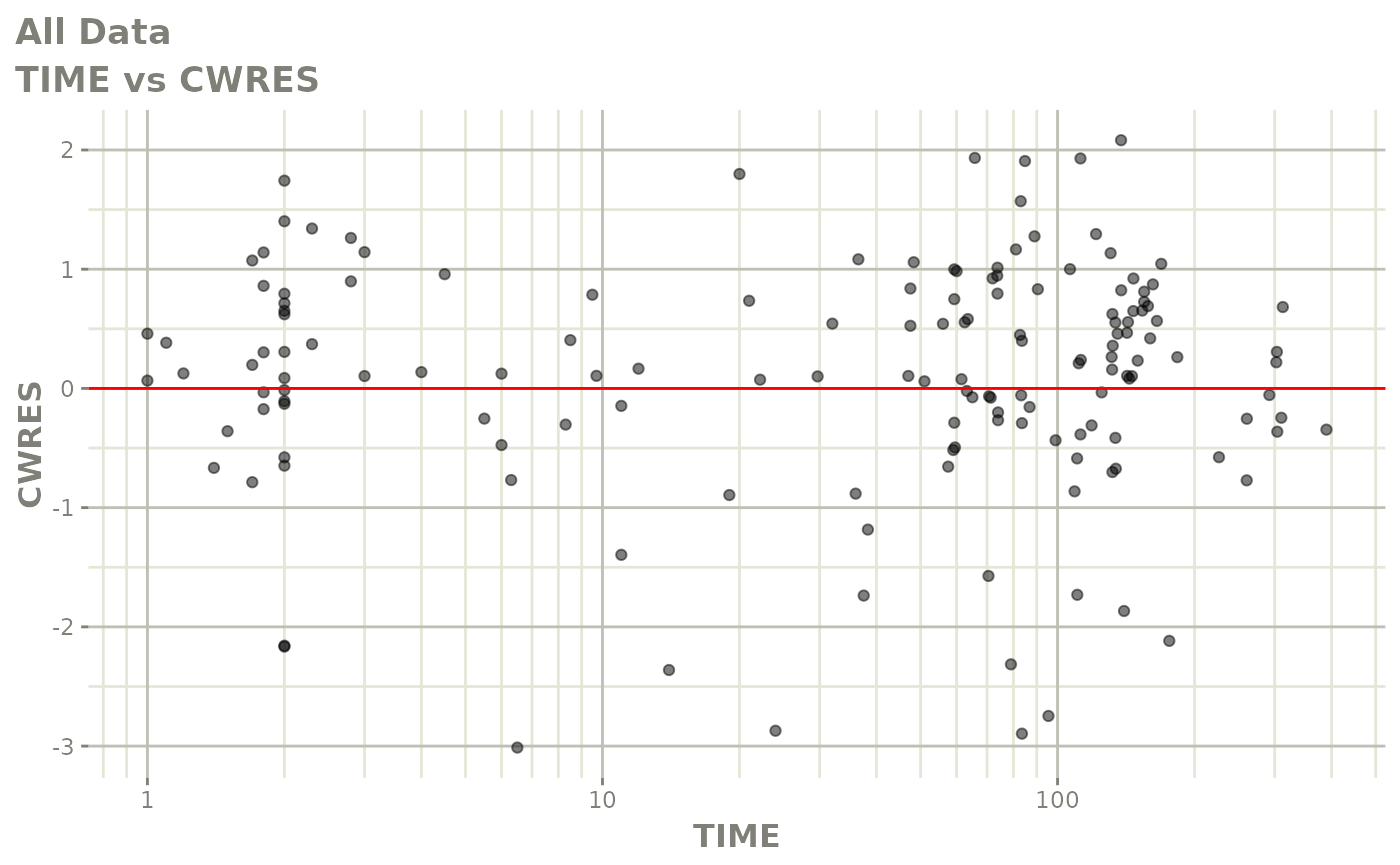
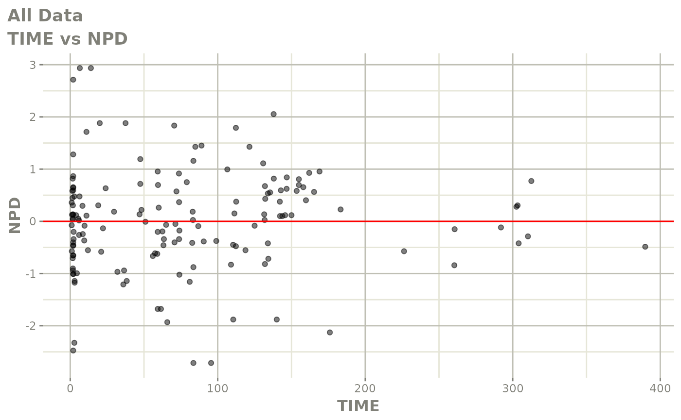
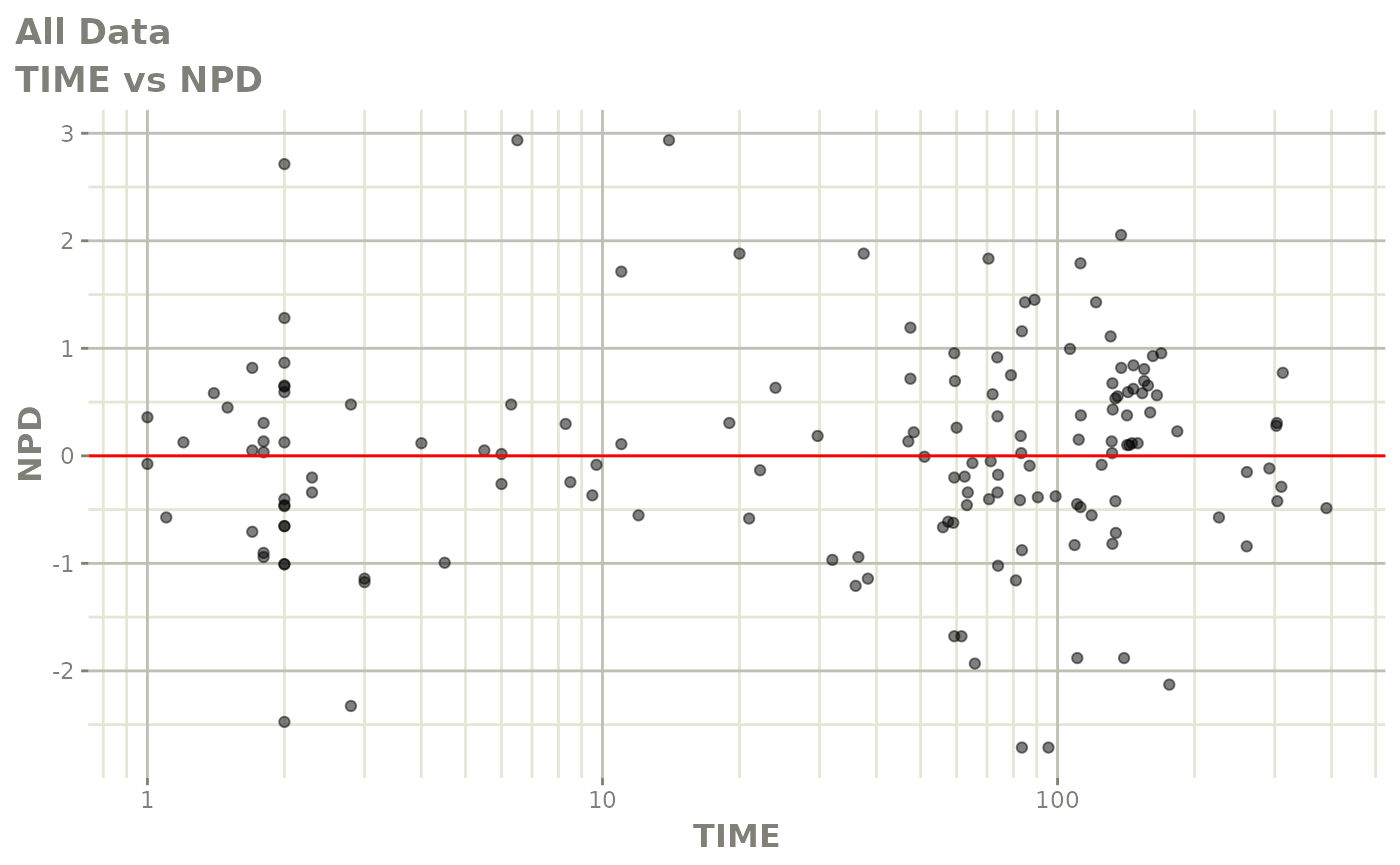
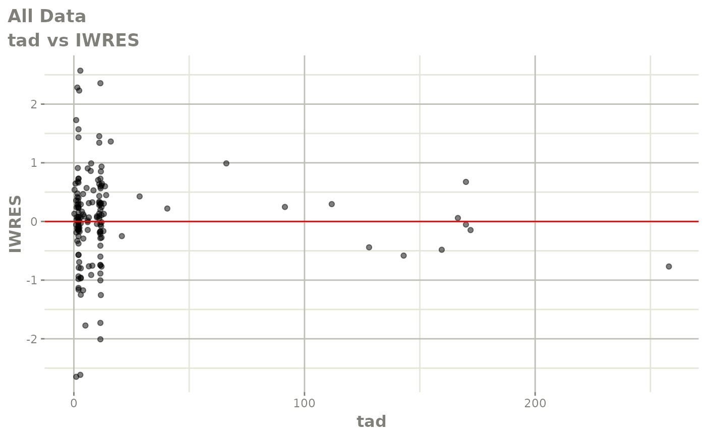
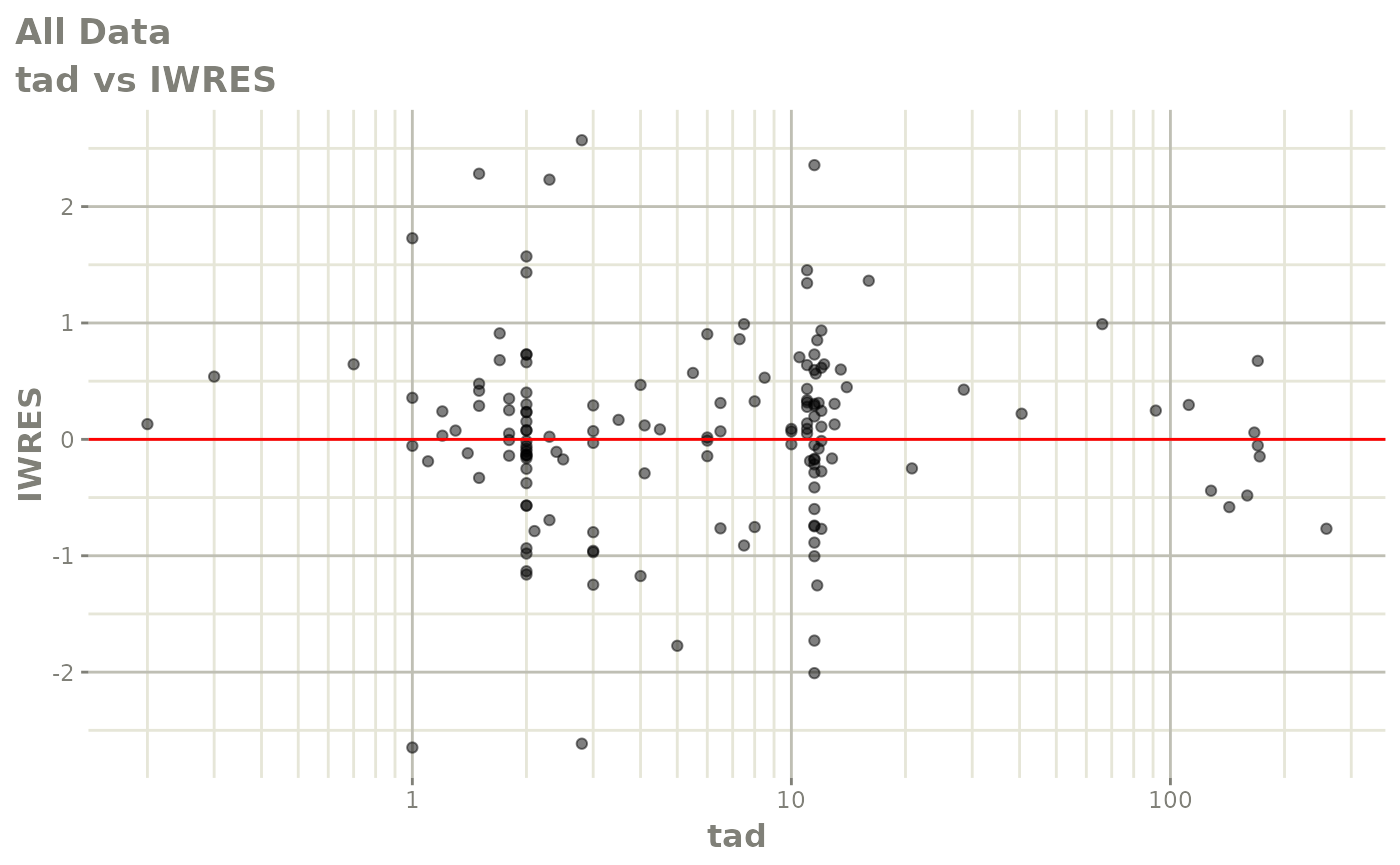
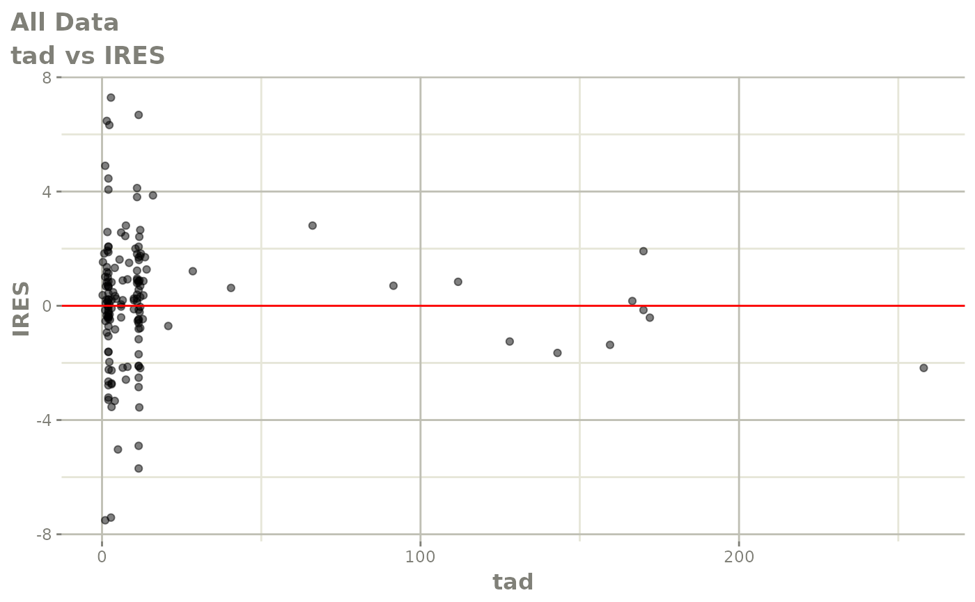
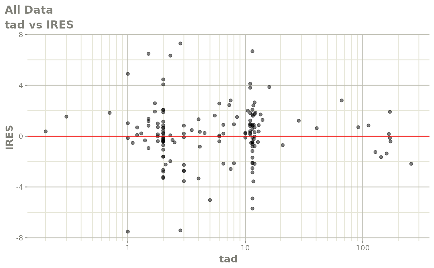
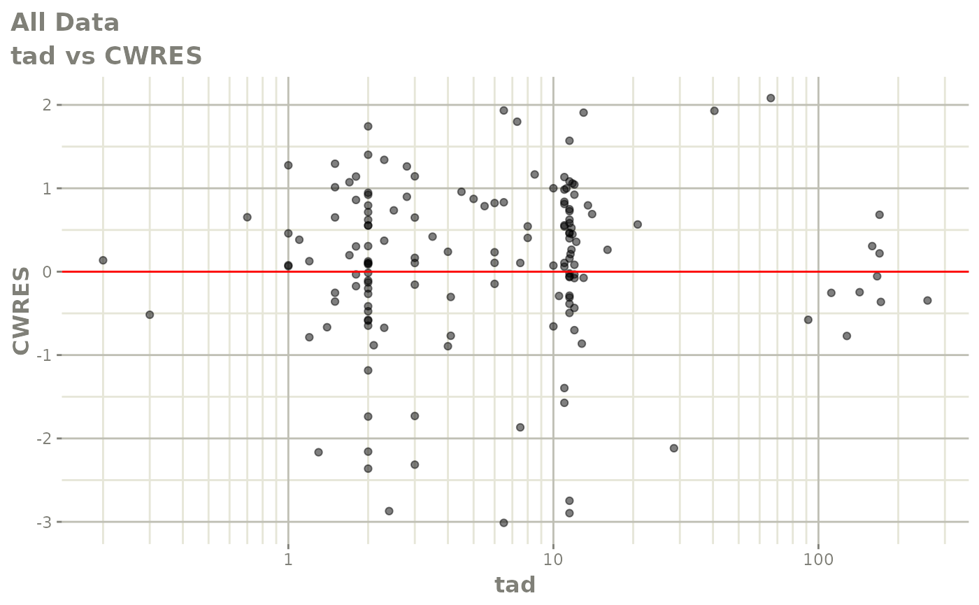
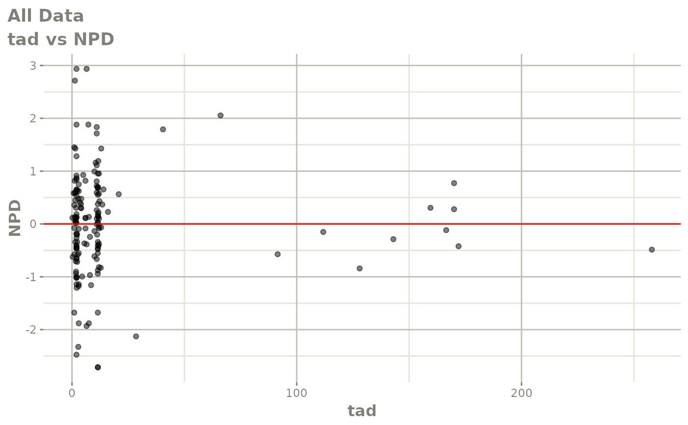
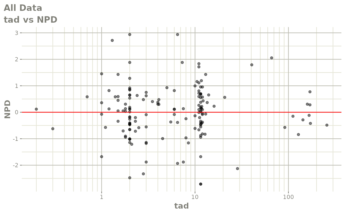
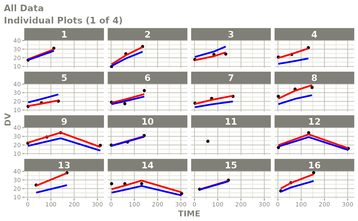
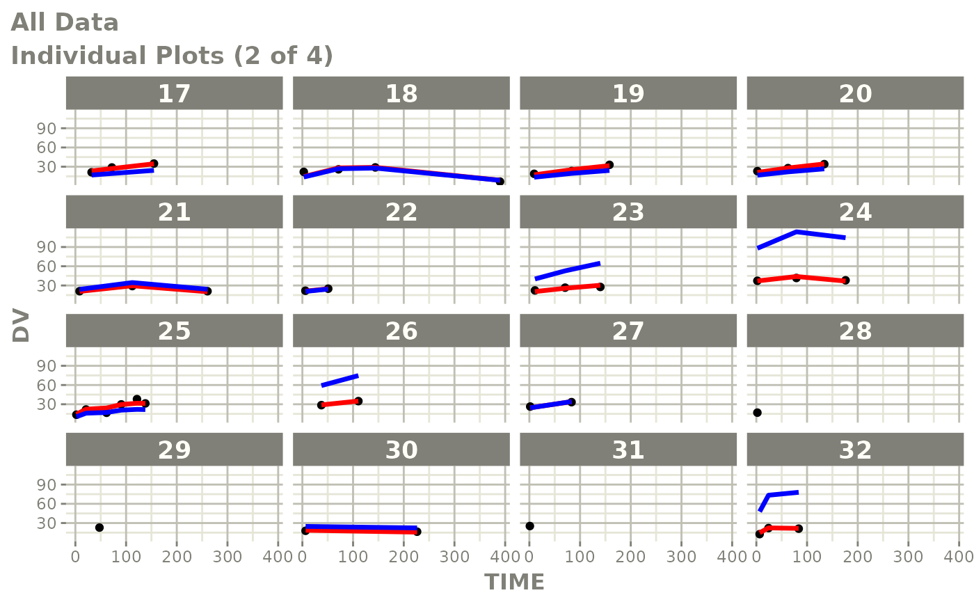
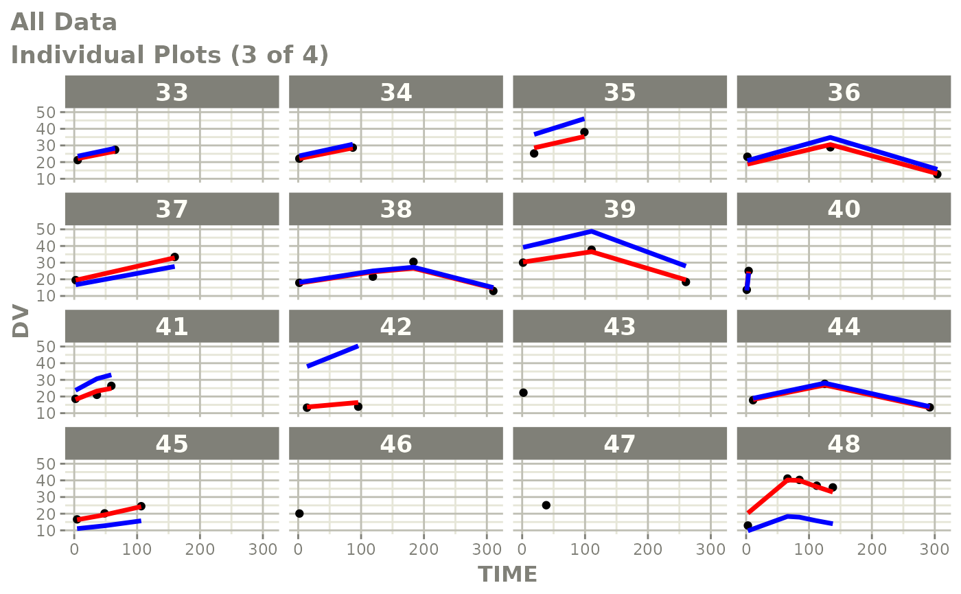
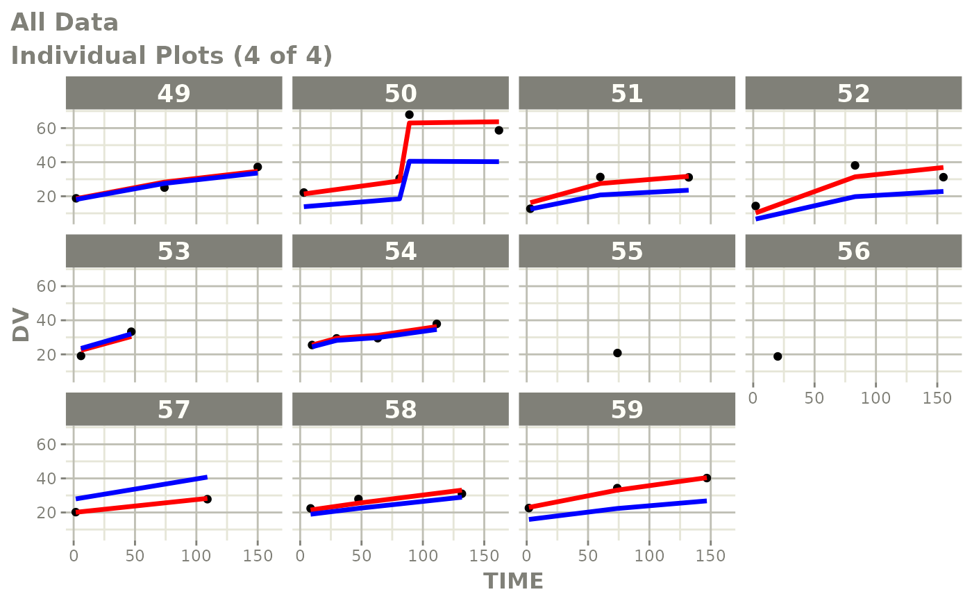
Those individual plots are not that great, it would be better to see the actual curves; You can with augPred

plot(augPred(fit))

Two types of VPCs

library(ggplot2)
p1 <- nlmixr::vpc(fit, show=list(obs_dv=TRUE));
p1 <- p1+ ylab("Concentrations")

## A prediction-corrected VPC
p2 <- nlmixr::vpc(fit, pred_corr = TRUE, show=list(obs_dv=TRUE))
p2 <- p2+ ylab("Prediction-Corrected Concentrations")

library(patchwork)
p1 / p2