Working with multiple endpoints
2022-03-26
Source:vignettes/multiple-endpoints.Rmd
multiple-endpoints.Rmdnlmixr
Multiple endpoints
Joint PK/PD models, or PK/PD models where you fix certain components are common in pharmacometrics. A classic example, (provided by Tomoo Funaki and Nick Holford) is Warfarin.
In this example, we have a transit-compartment (from depot to gut to central volume) PK model and an effect compartment for the PCA measurement.
Below is an illustrated example of a model that can be applied to the data:
pk.turnover.emax <- function() {
  ini({
    tktr <- log(1)
    tka <- log(1)
    tcl <- log(0.1)
    tv <- log(10)
    ##
    eta.ktr ~ 1
    eta.ka ~ 1
    eta.cl ~ 2
    eta.v ~ 1
    prop.err <- 0.1
    pkadd.err <- 0.1
    ##
    temax <- logit(0.8)
    #temax <- 7.5
    tec50 <- log(0.5)
    tkout <- log(0.05)
    te0 <- log(100)
    ##
    eta.emax ~ .5
    eta.ec50  ~ .5
    eta.kout ~ .5
    eta.e0 ~ .5
    ##
    pdadd.err <- 10
  })
  model({
    ktr <- exp(tktr + eta.ktr)
    ka <- exp(tka + eta.ka)
    cl <- exp(tcl + eta.cl)
    v <- exp(tv + eta.v)
    ##
    #poplogit = log(temax/(1-temax))
    emax=expit(temax+eta.emax)
    #logit=temax+eta.emax
    ec50 =  exp(tec50 + eta.ec50)
    kout = exp(tkout + eta.kout)
    e0 = exp(te0 + eta.e0)
    ##
    DCP = center/v
    PD=1-emax*DCP/(ec50+DCP)
    ##
    effect(0) = e0
    kin = e0*kout
    ##
    d/dt(depot) = -ktr * depot
    d/dt(gut) =  ktr * depot -ka * gut
    d/dt(center) =  ka * gut - cl / v * center
    d/dt(effect) = kin*PD -kout*effect
    ##
    cp = center / v
    cp ~ prop(prop.err) + add(pkadd.err)
    effect ~ add(pdadd.err)
  })
}
Notice there are two endpoints in the model cp and effect. Both are modeled in nlmixr using the ~ “modeled by” specification.
To see more about how nlmixr will handle the multiple compartment model, it is quite informative to parse the model and print the information about that model. In this case an initial parsing would give:
ui <- nlmixr(pk.turnover.emax)
ui
#> ▂▂ RxODE-based ODE model ▂▂▂▂▂▂▂▂▂▂▂▂▂▂▂▂▂▂▂▂▂▂▂▂▂▂▂▂▂▂▂▂▂▂▂▂▂▂▂▂▂▂▂▂▂▂▂▂▂▂▂▂▂▂▂
#> ── Initialization: ─────────────────────────────────────────────────────────────
#> Fixed Effects ($theta):
#>       tktr        tka        tcl         tv      temax      tec50      tkout
#>  0.0000000  0.0000000 -2.3025851  2.3025851  1.3862944 -0.6931472 -2.9957323
#>        te0
#>  4.6051702
#>
#> Omega ($omega):
#>          eta.ktr eta.ka eta.cl eta.v eta.emax eta.ec50 eta.kout eta.e0
#> eta.ktr        1      0      0     0      0.0      0.0      0.0    0.0
#> eta.ka         0      1      0     0      0.0      0.0      0.0    0.0
#> eta.cl         0      0      2     0      0.0      0.0      0.0    0.0
#> eta.v          0      0      0     1      0.0      0.0      0.0    0.0
#> eta.emax       0      0      0     0      0.5      0.0      0.0    0.0
#> eta.ec50       0      0      0     0      0.0      0.5      0.0    0.0
#> eta.kout       0      0      0     0      0.0      0.0      0.5    0.0
#> eta.e0         0      0      0     0      0.0      0.0      0.0    0.5
#> ── Multiple Endpoint Model ($multipleEndpoint): ────────────────────────────────
#> ┌─────────────────────────┬─────────────────────────┬─────────────────────────┐
#> │ variable                │ cmt                     │ dvid*                   │
#> ├─────────────────────────┼─────────────────────────┼─────────────────────────┤
#> │ variable                │ cmt                     │ dvid*                   │
#> ├─────────────────────────┼─────────────────────────┼─────────────────────────┤
#> │ cp ~ …                  │ cmt='cp' or cmt=5       │ dvid='cp' or dvid=1     │
#> ├─────────────────────────┼─────────────────────────┼─────────────────────────┤
#> │ effect ~ …              │ cmt='effect' or cmt=4   │ dvid='effect' or dvid=2 │
#> └─────────────────────────┴─────────────────────────┴─────────────────────────┘
#>   * If dvids are outside this range, all dvids are re-numered
#>   sequentially, ie 1,7, 10 becomes 1,2,3 etc
#>
#> ── μ-referencing ($muRefTable): ────────────────────────────────────────────────
#>                              ┌─────────┬──────────┐
#>                              │ theta   │ eta      │
#>                              ├─────────┼──────────┤
#>                              │ tktr    │ eta.ktr  │
#>                              ├─────────┼──────────┤
#>                              │ tka     │ eta.ka   │
#>                              ├─────────┼──────────┤
#>                              │ tcl     │ eta.cl   │
#>                              ├─────────┼──────────┤
#>                              │ tv      │ eta.v    │
#>                              ├─────────┼──────────┤
#>                              │ temax   │ eta.emax │
#>                              ├─────────┼──────────┤
#>                              │ tec50   │ eta.ec50 │
#>                              ├─────────┼──────────┤
#>                              │ tkout   │ eta.kout │
#>                              ├─────────┼──────────┤
#>                              │ te0     │ eta.e0   │
#>                              └─────────┴──────────┘
#>
#> ── Model: ──────────────────────────────────────────────────────────────────────
#>     ktr <- exp(tktr + eta.ktr)
#>     ka <- exp(tka + eta.ka)
#>     cl <- exp(tcl + eta.cl)
#>     v <- exp(tv + eta.v)
#>     ##
#>     #poplogit = log(temax/(1-temax))
#>     emax=expit(temax+eta.emax)
#>     #logit=temax+eta.emax
#>     ec50 =  exp(tec50 + eta.ec50)
#>     kout = exp(tkout + eta.kout)
#>     e0 = exp(te0 + eta.e0)
#>     ##
#>     DCP = center/v
#>     PD=1-emax*DCP/(ec50+DCP)
#>     ##
#>     effect(0) = e0
#>     kin = e0*kout
#>     ##
#>     d/dt(depot) = -ktr * depot
#>     d/dt(gut) =  ktr * depot -ka * gut
#>     d/dt(center) =  ka * gut - cl / v * center
#>     d/dt(effect) = kin*PD -kout*effect
#>     ##
#>     cp = center / v
#>     cp ~ prop(prop.err) + add(pkadd.err)
#>     effect ~ add(pdadd.err)
#> ▂▂▂▂▂▂▂▂▂▂▂▂▂▂▂▂▂▂▂▂▂▂▂▂▂▂▂▂▂▂▂▂▂▂▂▂▂▂▂▂▂▂▂▂▂▂▂▂▂▂▂▂▂▂▂▂▂▂▂▂▂▂▂▂▂▂▂▂▂▂▂▂▂▂▂▂▂▂▂▂
In the middle of the printout, it shows how the data must be formatted (using the cmt and dvid data items) to allow nlmixr to model the multiple endpoint appropriately.
Of course if you are interested you can directly access the information in ui$multipleEndpoint.
ui$multipleEndpoint| variable | cmt | dvid* |
|---|---|---|
| variable | cmt | dvid* |
| cp ~ … | cmt='cp' or cmt=5 | dvid='cp' or dvid=1 |
| effect ~ … | cmt='effect' or cmt=4 | dvid='effect' or dvid=2 |
| * If dvids are outside this range, all dvids are re-numered sequentially, ie 1,7, 10 becomes 1,2,3 etc | ||
Notice that the cmt and dvid items can use the named variables directly as either the cmt or dvid specification. This flexible notation makes it so you do not have to rename your compartments to run nlmixr model functions.
The other thing to note is that the cp is specified by an ODE compartment above the number of compartments defined in the RxODE part of the nlmixr model. This is because cp is not a defined compartment, but a related variable cp.
The last thing to notice that the cmt items are numbered cmt=5 for cp or cmt=4 for effect even though they were specified in the model first by cp and cmt. This ordering is because effect is a compartment in the RxODE system. Of course cp is related to the compartment central, and it may make more sense to pair cp with the central compartment.
If this is something you want to have you can specify the compartment to relate the effect to by the | operator. In this case you would change
cp ~ prop(prop.err) + add(pkadd.err)to
cp ~ prop(prop.err) + add(pkadd.err) | centralWith this change, the model could be updated to:
pk.turnover.emax2 <- function() {
  ini({
    tktr <- log(1)
    tka <- log(1)
    tcl <- log(0.1)
    tv <- log(10)
    ##
    eta.ktr ~ 1
    eta.ka ~ 1
    eta.cl ~ 2
    eta.v ~ 1
    prop.err <- 0.1
    pkadd.err <- 0.1
    ##
    temax <- logit(0.8)
    tec50 <- log(0.5)
    tkout <- log(0.05)
    te0 <- log(100)
    ##
    eta.emax ~ .5
    eta.ec50  ~ .5
    eta.kout ~ .5
    eta.e0 ~ .5
    ##
    pdadd.err <- 10
  })
  model({
    ktr <- exp(tktr + eta.ktr)
    ka <- exp(tka + eta.ka)
    cl <- exp(tcl + eta.cl)
    v <- exp(tv + eta.v)
    ##
    emax=expit(temax+eta.emax)
    ec50 =  exp(tec50 + eta.ec50)
    kout = exp(tkout + eta.kout)
    e0 = exp(te0 + eta.e0)
    ##
    DCP = center/v
    PD=1-emax*DCP/(ec50+DCP)
    ##
    effect(0) = e0
    kin = e0*kout
    ##
    d/dt(depot) = -ktr * depot
    d/dt(gut) =  ktr * depot -ka * gut
    d/dt(center) =  ka * gut - cl / v * center
    d/dt(effect) = kin*PD -kout*effect
    ##
    cp = center / v
    cp ~ prop(prop.err) + add(pkadd.err) | center
    effect ~ add(pdadd.err)
  })
}
ui2 <- nlmixr(pk.turnover.emax2)
ui2$multipleEndpoint| variable | cmt | dvid* |
|---|---|---|
| variable | cmt | dvid* |
| cp ~ … | cmt='center' or cmt=3 | dvid='center' or dvid=1 |
| effect ~ … | cmt='effect' or cmt=4 | dvid='effect' or dvid=2 |
| * If dvids are outside this range, all dvids are re-numered sequentially, ie 1,7, 10 becomes 1,2,3 etc | ||
Notice in this case the cmt variables are numbered sequentially and the cp variable matches the center compartment.
DVID vs CMT, which one is used
When dvid and cmt are combined in the same dataset, the cmt data item is always used on the event information and the dvid is used on the observations. nlmixr expects the cmt data item to match the dvid item for observations OR to be either zero or one for the dvid to replace the cmt information.
If you do not wish to use dvid items to define multiple endpoints in nlmixr, you can set the following option:
options(RxODE.combine.dvid=FALSE)
ui2$multipleEndpoint| variable | cmt |
|---|---|
| variable | cmt |
| cp ~ … | cmt='center' or cmt=3 |
| effect ~ … | cmt='effect' or cmt=4 |
Then only cmt items are used for the multiple endpoint models. Of course you can turn it on or off for different models if you wish:
options(RxODE.combine.dvid=TRUE)
ui2$multipleEndpoint| variable | cmt | dvid* |
|---|---|---|
| variable | cmt | dvid* |
| cp ~ … | cmt='center' or cmt=3 | dvid='center' or dvid=1 |
| effect ~ … | cmt='effect' or cmt=4 | dvid='effect' or dvid=2 |
| * If dvids are outside this range, all dvids are re-numered sequentially, ie 1,7, 10 becomes 1,2,3 etc | ||
Running a multiple endpoint model
With this information, we can use the built-in warfarin dataset in nlmixr:
summary(warfarin)
#>        id             time             amt                dv          dvid
#>  Min.   : 1.00   Min.   :  0.00   Min.   :  0.000   Min.   :  0.00   cp :283
#>  1st Qu.: 8.00   1st Qu.: 24.00   1st Qu.:  0.000   1st Qu.:  4.50   pca:232
#>  Median :15.00   Median : 48.00   Median :  0.000   Median : 11.40
#>  Mean   :16.08   Mean   : 52.08   Mean   :  6.524   Mean   : 20.02
#>  3rd Qu.:24.00   3rd Qu.: 96.00   3rd Qu.:  0.000   3rd Qu.: 26.00
#>  Max.   :33.00   Max.   :144.00   Max.   :153.000   Max.   :100.00
#>       evid               wt              age            sex
#>  Min.   :0.00000   Min.   : 40.00   Min.   :21.00   female:101
#>  1st Qu.:0.00000   1st Qu.: 60.00   1st Qu.:23.00   male  :414
#>  Median :0.00000   Median : 70.00   Median :28.00
#>  Mean   :0.06214   Mean   : 69.27   Mean   :31.85
#>  3rd Qu.:0.00000   3rd Qu.: 78.00   3rd Qu.:36.00
#>  Max.   :1.00000   Max.   :102.00   Max.   :63.00
Since dvid specifies pca as the effect endpoint, you can update the model to be more explicit making one last change:
cp ~ prop(prop.err) + add(pkadd.err)
effect ~ add(pdadd.err)
to
cp ~ prop(prop.err) + add(pkadd.err)
effect ~ add(pdadd.err)  | pca
pk.turnover.emax3 <- function() {
  ini({
    tktr <- log(1)
    tka <- log(1)
    tcl <- log(0.1)
    tv <- log(10)
    ##
    eta.ktr ~ 1
    eta.ka ~ 1
    eta.cl ~ 2
    eta.v ~ 1
    prop.err <- 0.1
    pkadd.err <- 0.1
    ##
    temax <- logit(0.8)
    tec50 <- log(0.5)
    tkout <- log(0.05)
    te0 <- log(100)
    ##
    eta.emax ~ .5
    eta.ec50  ~ .5
    eta.kout ~ .5
    eta.e0 ~ .5
    ##
    pdadd.err <- 10
  })
  model({
    ktr <- exp(tktr + eta.ktr)
    ka <- exp(tka + eta.ka)
    cl <- exp(tcl + eta.cl)
    v <- exp(tv + eta.v)
    emax = expit(temax+eta.emax)
    ec50 =  exp(tec50 + eta.ec50)
    kout = exp(tkout + eta.kout)
    e0 = exp(te0 + eta.e0)
    ##
    DCP = center/v
    PD=1-emax*DCP/(ec50+DCP)
    ##
    effect(0) = e0
    kin = e0*kout
    ##
    d/dt(depot) = -ktr * depot
    d/dt(gut) =  ktr * depot -ka * gut
    d/dt(center) =  ka * gut - cl / v * center
    d/dt(effect) = kin*PD -kout*effect
    ##
    cp = center / v
    cp ~ prop(prop.err) + add(pkadd.err)
    effect ~ add(pdadd.err) | pca
  })
}
Run the models with SAEM
fit.TOS <- nlmixr(pk.turnover.emax3, warfarin, "saem", control=list(print=0),
table=list(cwres=TRUE, npde=TRUE))
#> [====|====|====|====|====|====|====|====|====|====] 0:00:00
#>
#> [====|====|====|====|====|====|====|====|====|====] 0:00:00
#>
#> [====|====|====|====|====|====|====|====|====|====] 0:00:00
#>
#> [====|====|====|====|====|====|====|====|====|====] 0:00:00
#>
#> [====|====|====|====|====|====|====|====|====|====] 0:00:00
#>
#> [1] "CMT"
print(fit.TOS)
#> ── nlmixr SAEM(ODE); OBJF by FOCEi approximation fit ───────────────────────────
#>
#> OBJF AIC BIC Log-likelihood Condition Number
#> FOCEi 1381.827 2307.521 2386.942 -1134.761 1029.516
#>
#> ── Time (sec $time): ───────────────────────────────────────────────────────────
#>
#> saem setup table cwres covariance other
#> elapsed 87.73 12.38773 3.131 15.605 0.049 0.785272
#>
#> ── Population Parameters ($parFixed or $parFixedDf): ───────────────────────────
#>
#> Est. SE %RSE Back-transformed(95%CI) BSV(CV% or SD)
#> tktr 0.351 0.246 70 1.42 (0.878, 2.3) 110.
#> tka -0.079 0.157 198 0.924 (0.68, 1.26) 43.4
#> tcl -1.98 0.0511 2.58 0.138 (0.125, 0.153) 26.8
#> tv 2.01 0.0477 2.37 7.48 (6.81, 8.21) 21.9
#> prop.err 0.125 0.125
#> pkadd.err 0.718 0.718
#> temax 2.85 0.339 11.9 0.945 (0.899, 0.971) 0.120
#> tec50 -0.182 0.143 78.5 0.833 (0.63, 1.1) 50.0
#> tkout -2.89 0.037 1.28 0.0557 (0.0518, 0.0599) 6.01
#> te0 4.57 0.0114 0.249 96.6 (94.5, 98.8) 5.01
#> pdadd.err 3.8 3.8
#> Shrink(SD)%
#> tktr 53.0%
#> tka 65.0%
#> tcl 5.46%
#> tv 17.3%
#> prop.err
#> pkadd.err
#> temax 82.6%
#> tec50 9.40%
#> tkout 48.1%
#> te0 18.3%
#> pdadd.err
#>
#> Covariance Type ($covMethod): linFim
#> Some strong fixed parameter correlations exist ($cor) :
#> cor:tka,tktr cor:tcl,tktr cor:tv,tktr cor:temax,tktr cor:tec50,tktr
#> -0.232 -0.0211 0.0168 0.00532 -0.0134
#> cor:tkout,tktr cor:te0,tktr cor:tcl,tka cor:tv,tka cor:temax,tka
#> -0.0444 0.00180 -0.0226 0.0230 0.0344
#> cor:tec50,tka cor:tkout,tka cor:te0,tka cor:tv,tcl cor:temax,tcl
#> 0.0532 -0.00177 0.00604 0.0201 -0.0533
#> cor:tec50,tcl cor:tkout,tcl cor:te0,tcl cor:temax,tv cor:tec50,tv
#> -0.127 -0.0225 -0.0101 0.0883 0.105
#> cor:tkout,tv cor:te0,tv cor:tec50,temax cor:tkout,temax cor:te0,temax
#> 0.0559 0.0142 0.732 -0.758 -0.0227
#> cor:tkout,tec50 cor:te0,tec50 cor:te0,tkout
#> -0.470 -0.0652 0.110
#>
#>
#> No correlations in between subject variability (BSV) matrix
#> Full BSV covariance ($omega) or correlation ($omegaR; diagonals=SDs)
#> Distribution stats (mean/skewness/kurtosis/p-value) available in $shrink
#>
#> ── Fit Data (object is a modified tibble): ─────────────────────────────────────
#> # A tibble: 483 × 42
#> ID TIME CMT DV EPRED ERES NPDE NPD PRED RES WRES IPRED
#> <fct> <dbl> <fct> <dbl> <dbl> <dbl> <dbl> <dbl> <dbl> <dbl> <dbl> <dbl>
#> 1 1 0.5 cp 0 1.92 -1.92 0.583 0.583 1.50 -1.50 -1.05 0.501
#> 2 1 1 cp 1.9 4.61 -2.71 0.314 0.314 4.17 -2.27 -0.801 1.62
#> 3 1 2 cp 3.3 8.45 -5.15 -1.53 -1.53 8.65 -5.35 -1.42 4.31
#> # … with 480 more rows, and 30 more variables: IRES <dbl>, IWRES <dbl>,
#> # CPRED <dbl>, CRES <dbl>, CWRES <dbl>, eta.ktr <dbl>, eta.ka <dbl>,
#> # eta.cl <dbl>, eta.v <dbl>, eta.emax <dbl>, eta.ec50 <dbl>, eta.kout <dbl>,
#> # eta.e0 <dbl>, depot <dbl>, gut <dbl>, center <dbl>, effect <dbl>,
#> # ktr <dbl>, ka <dbl>, cl <dbl>, v <dbl>, emax <dbl>, ec50 <dbl>, kout <dbl>,
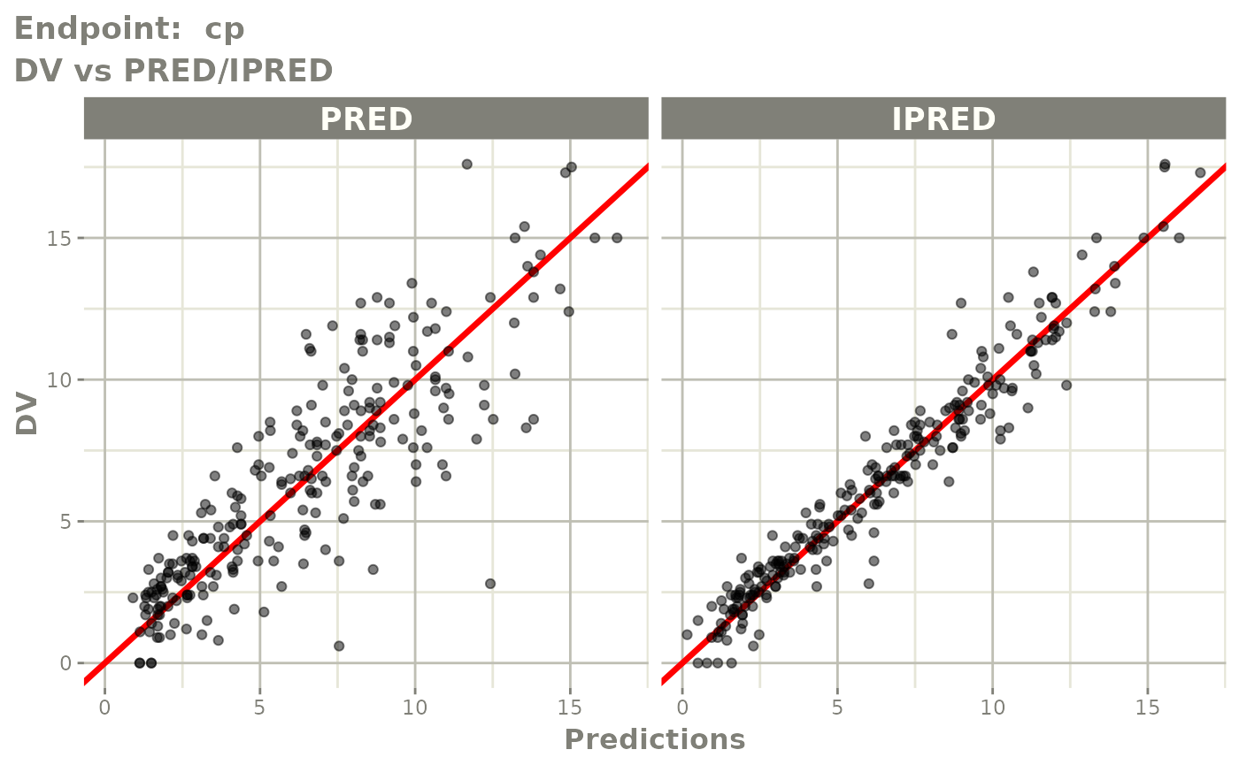
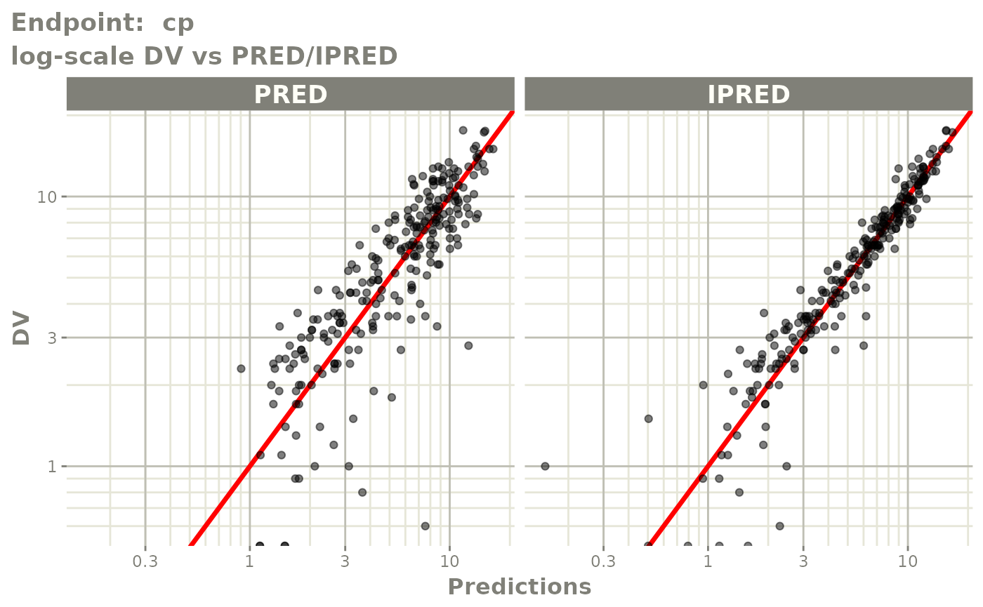
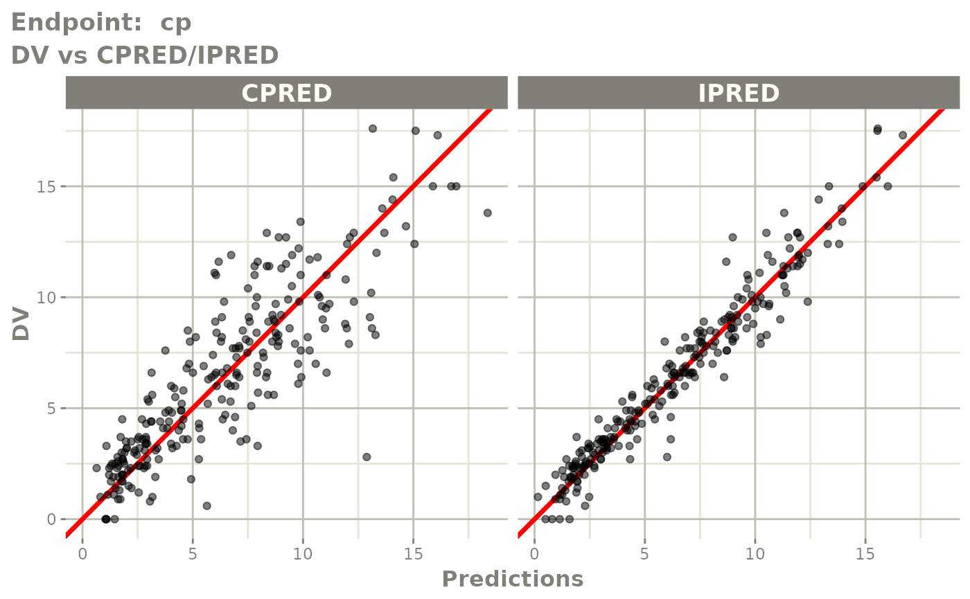
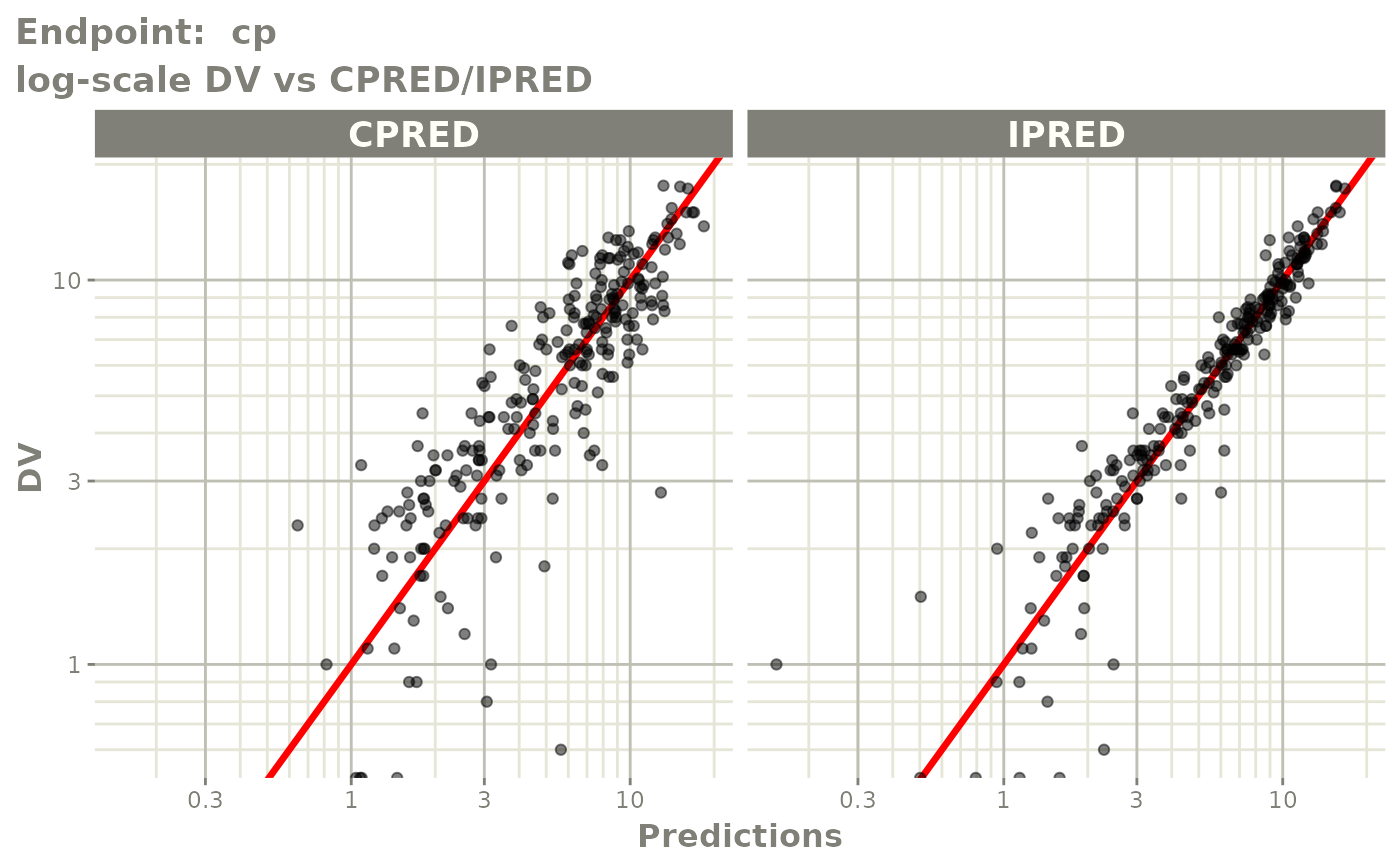
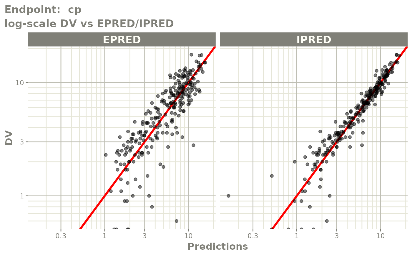
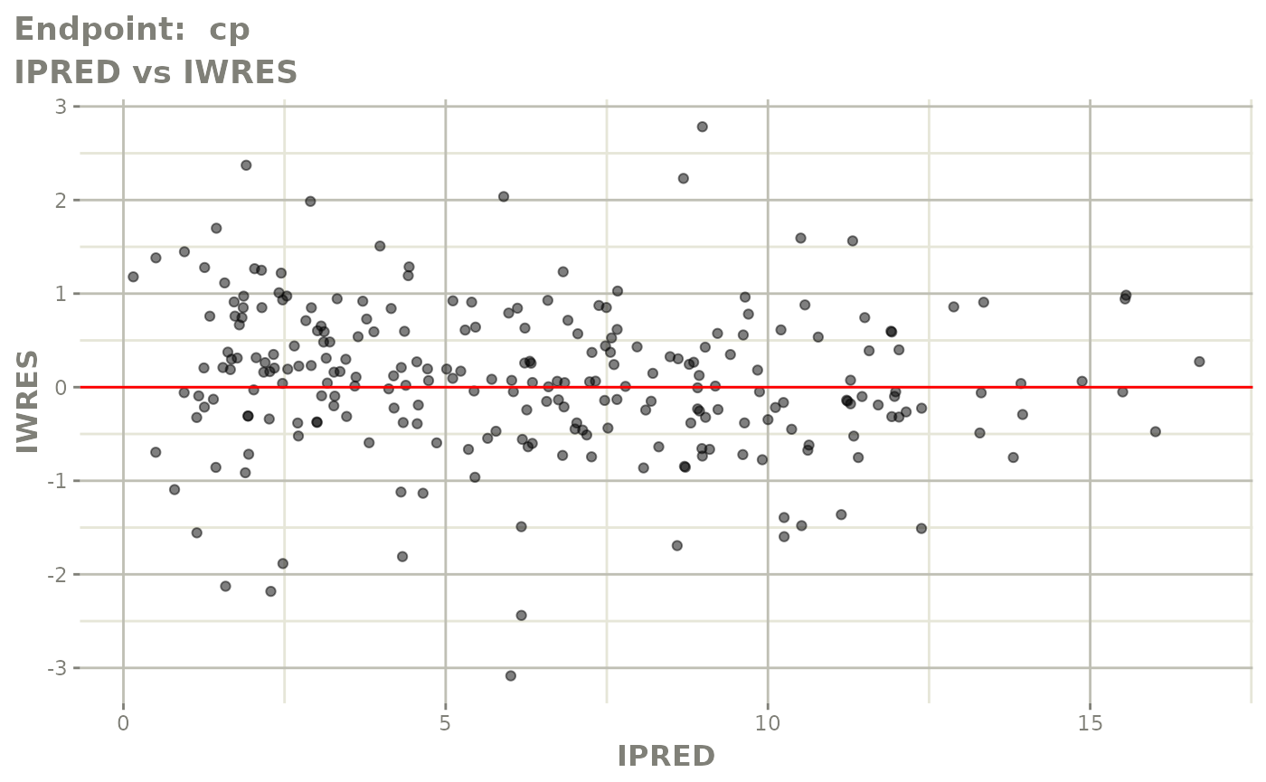
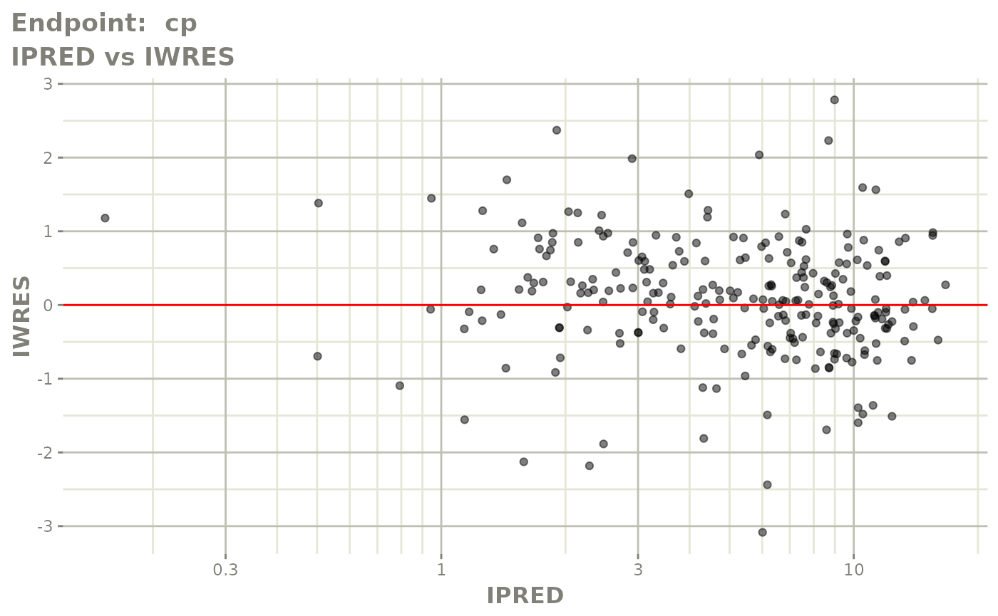
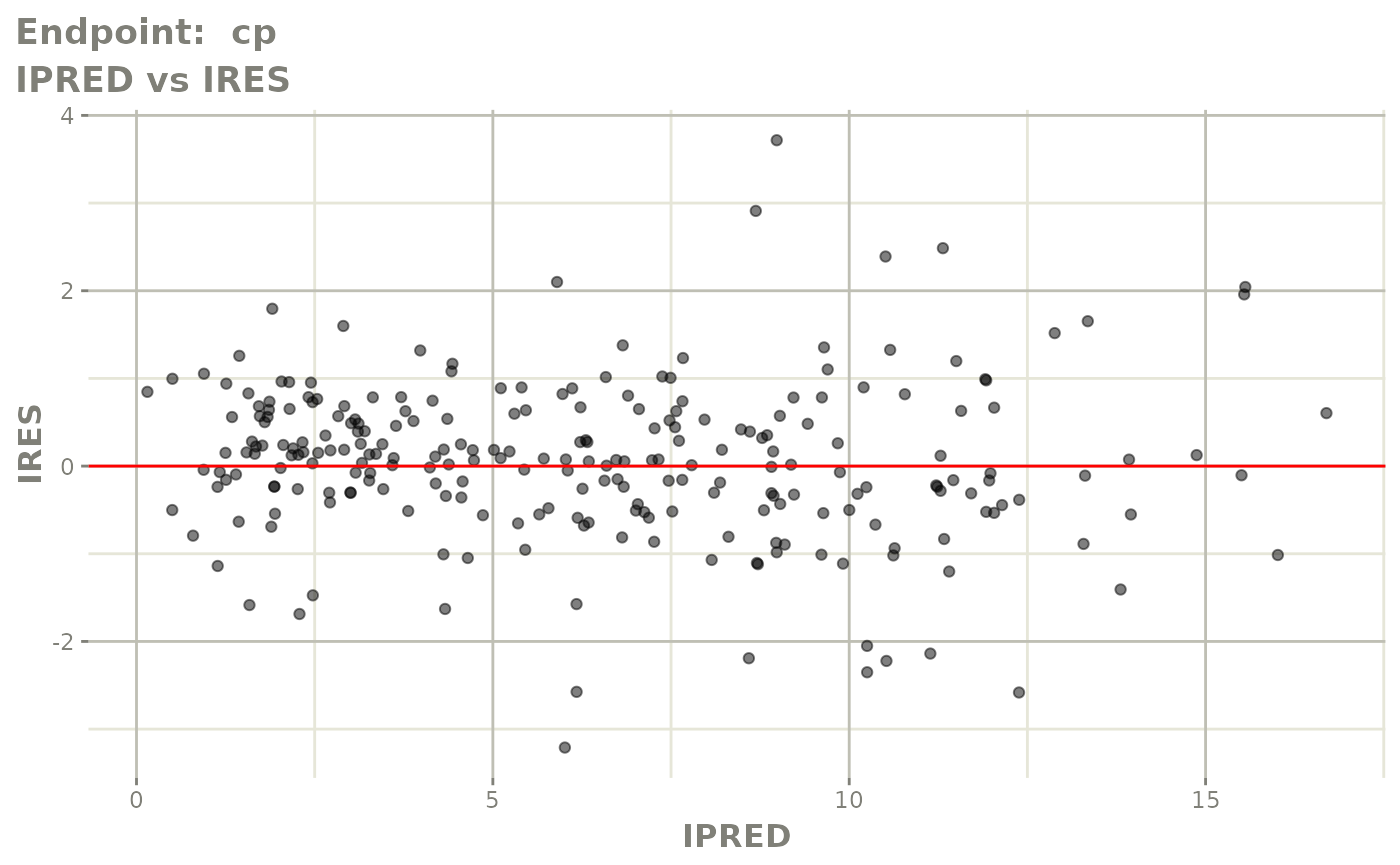
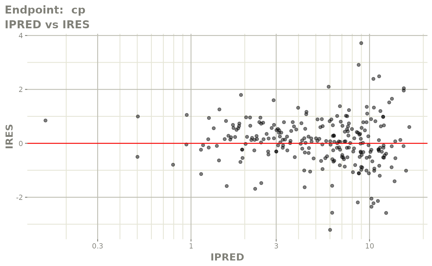
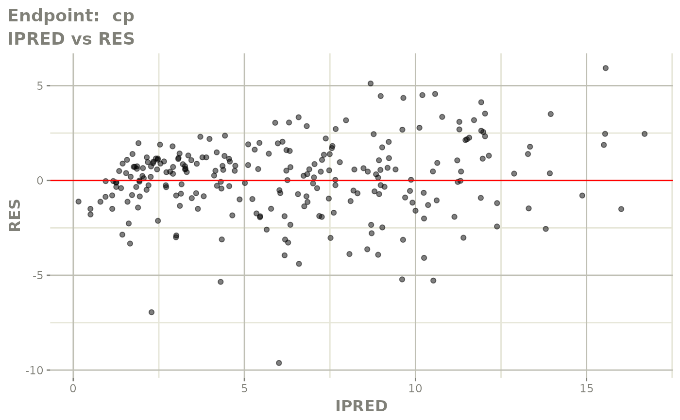
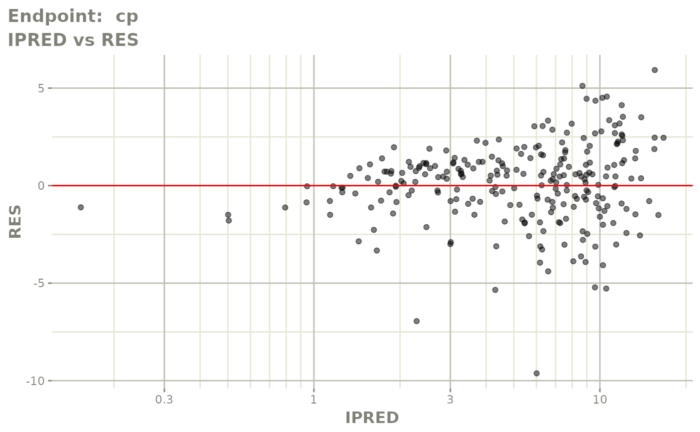
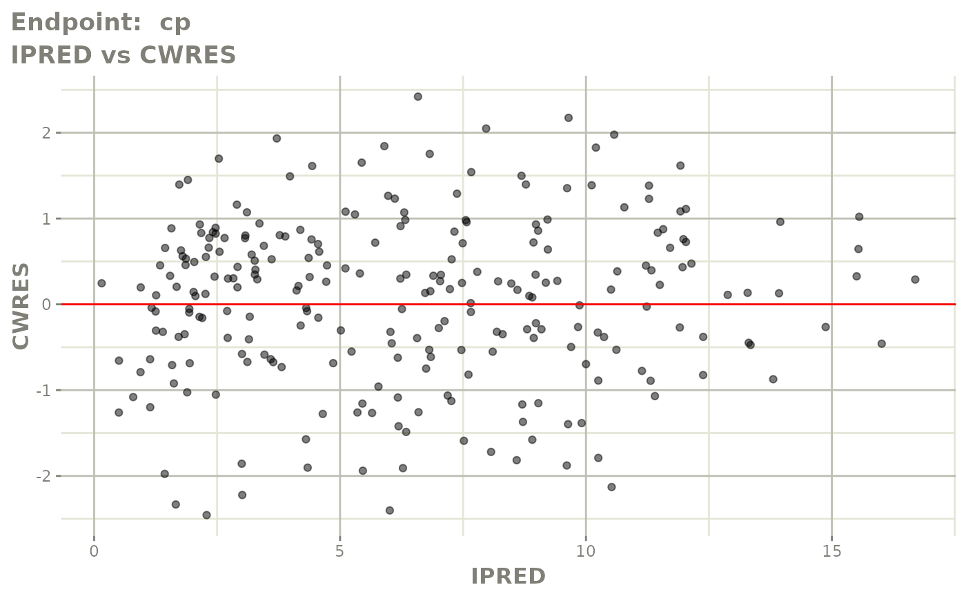
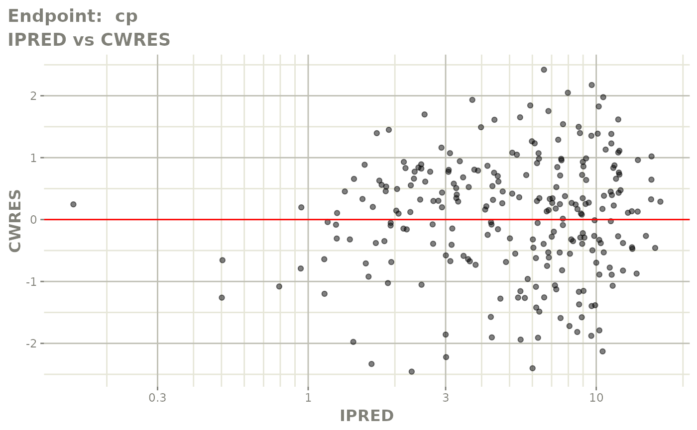
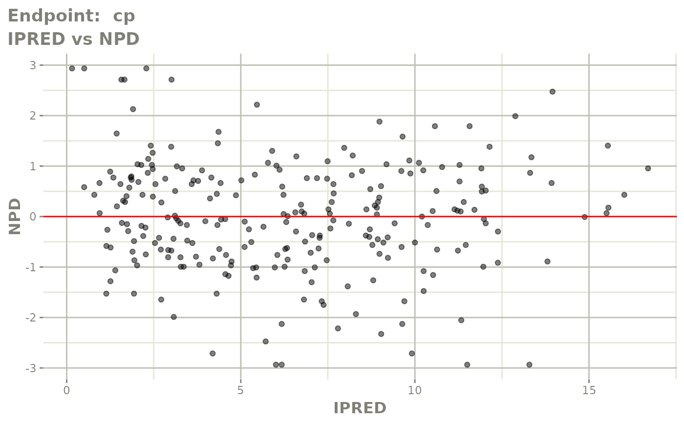
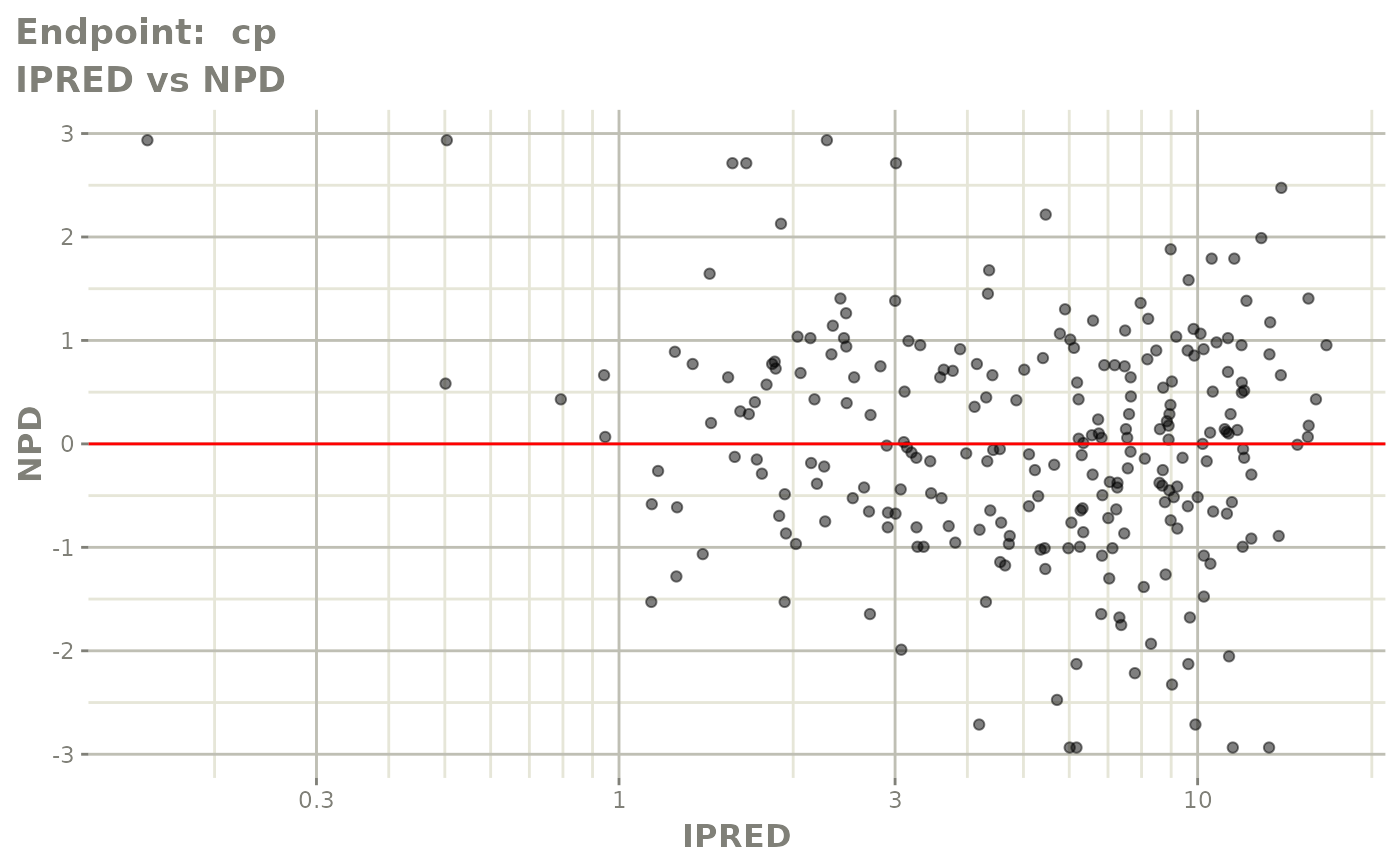
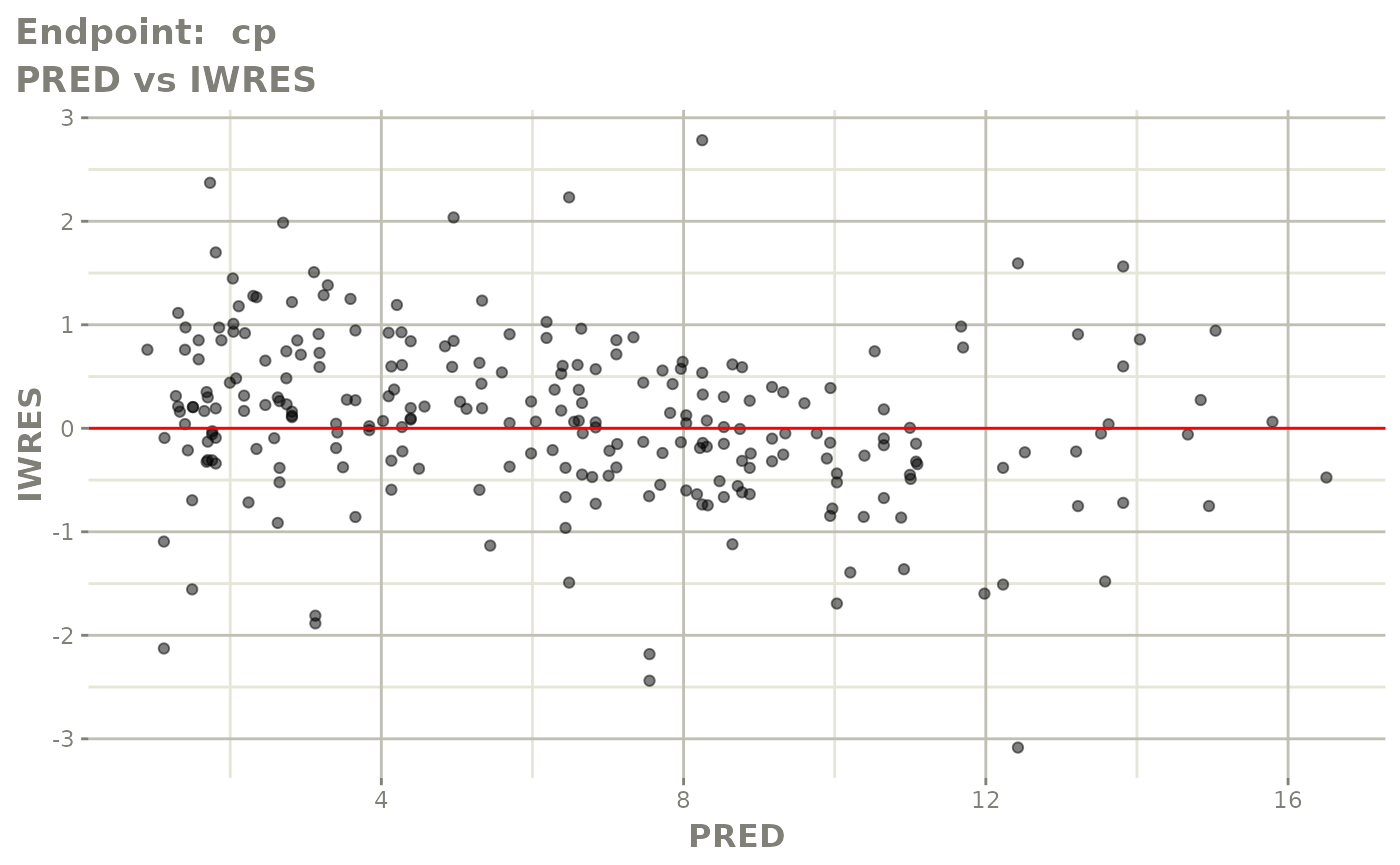
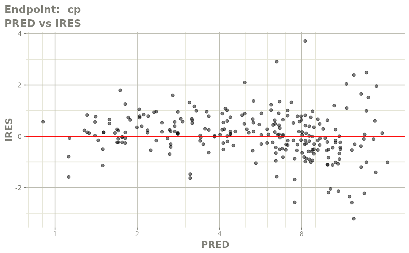
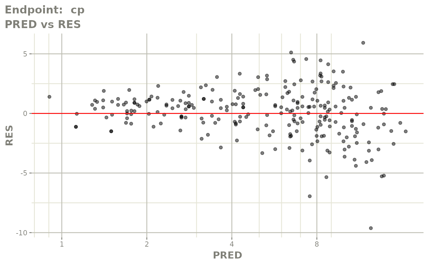
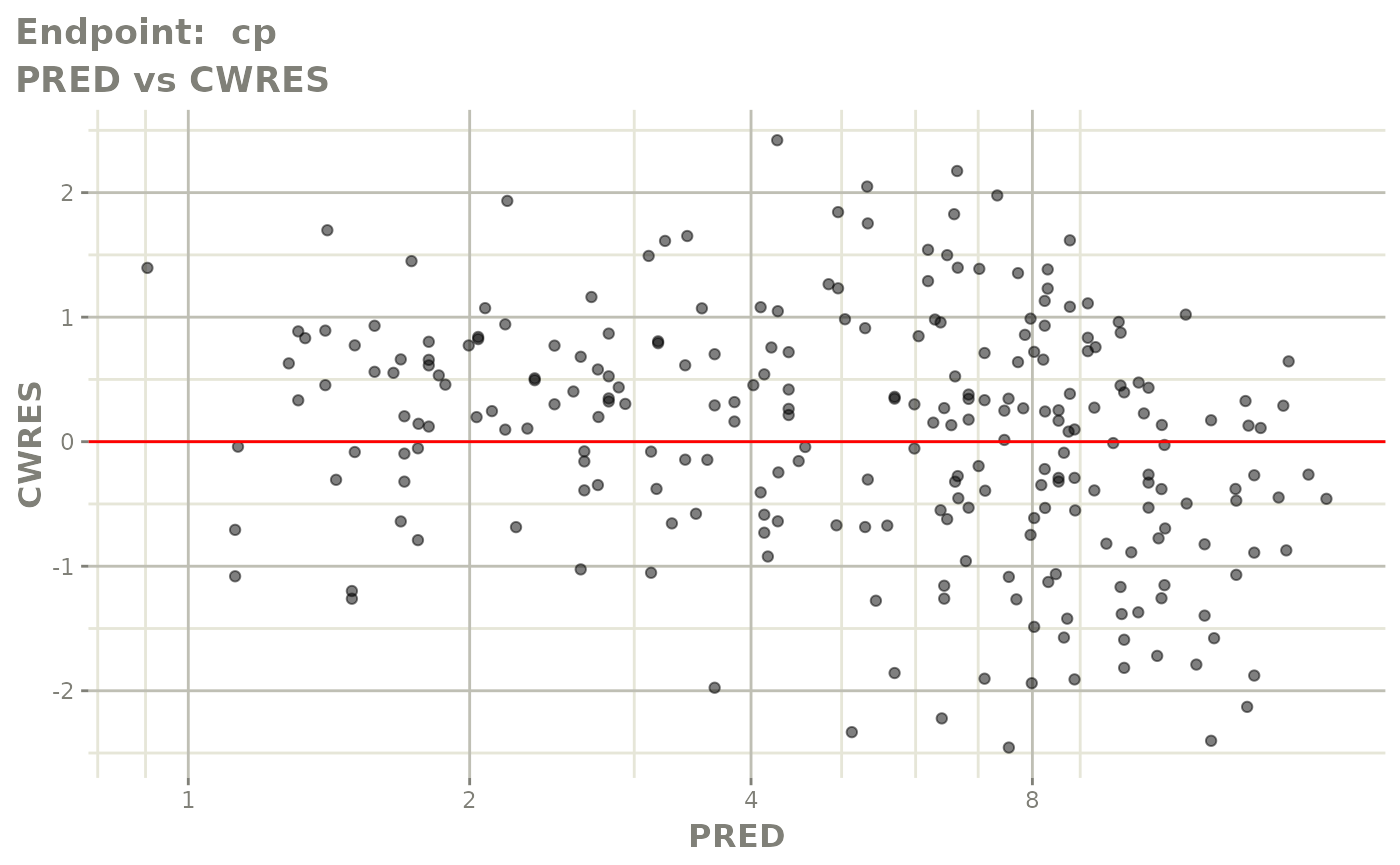
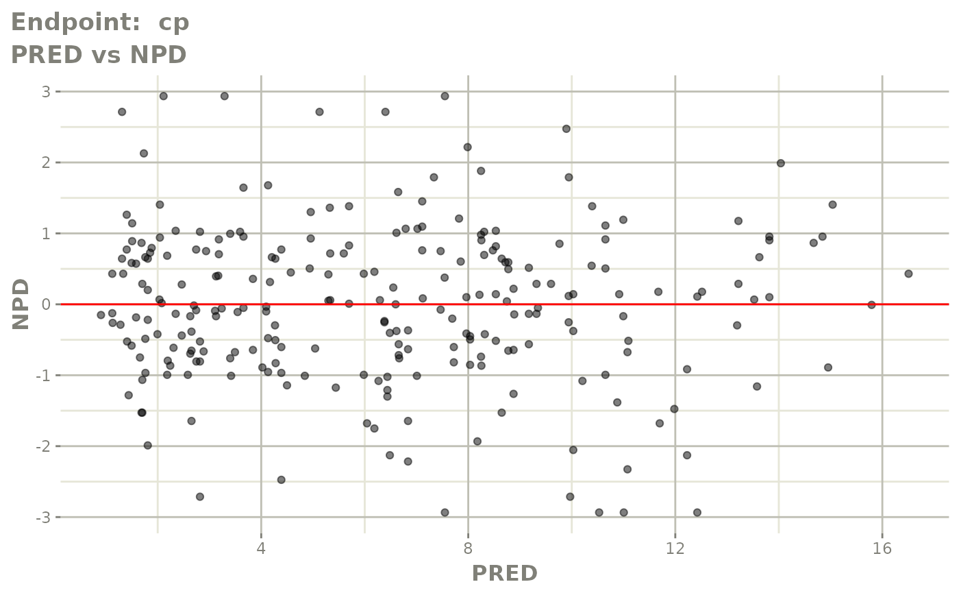
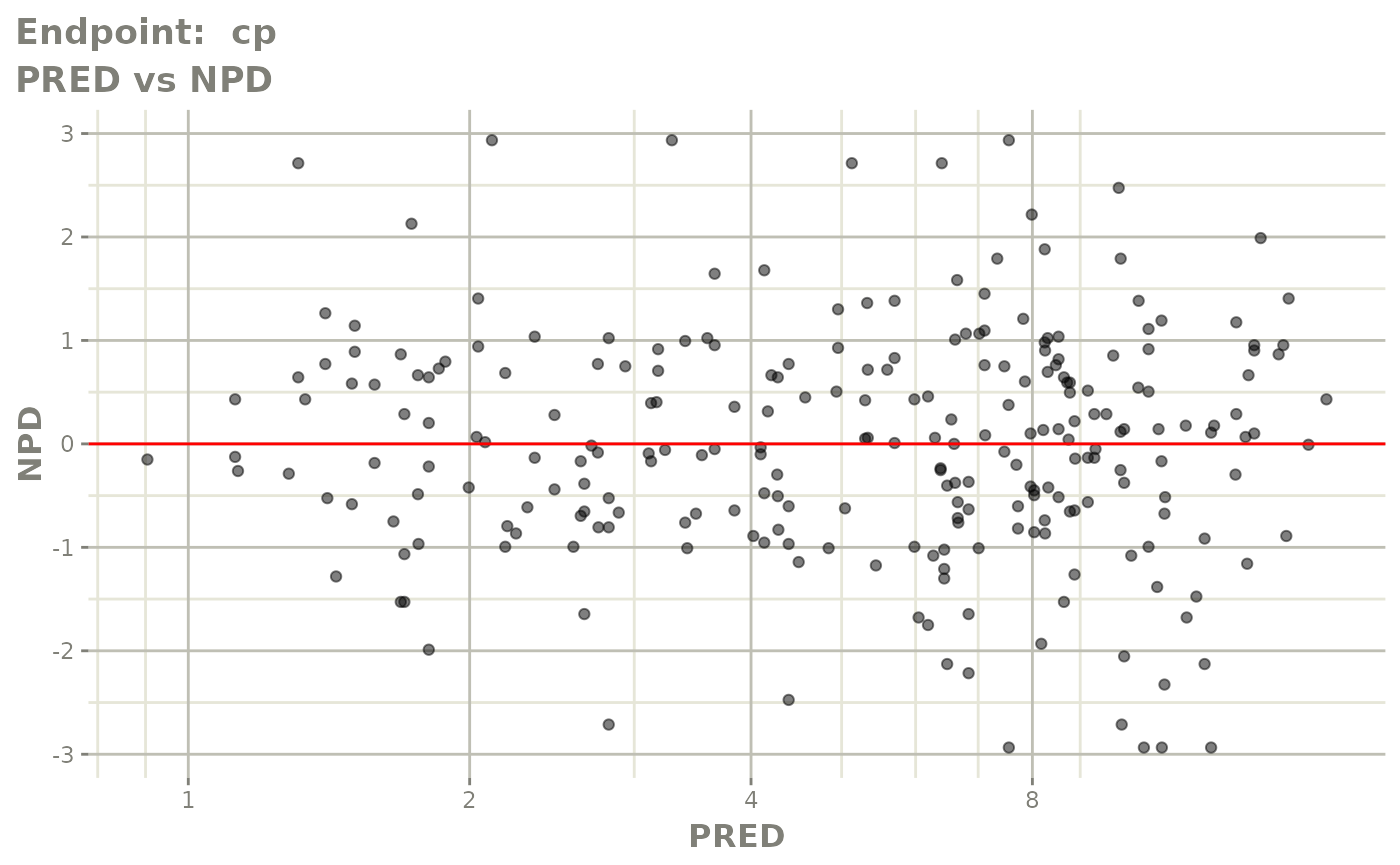
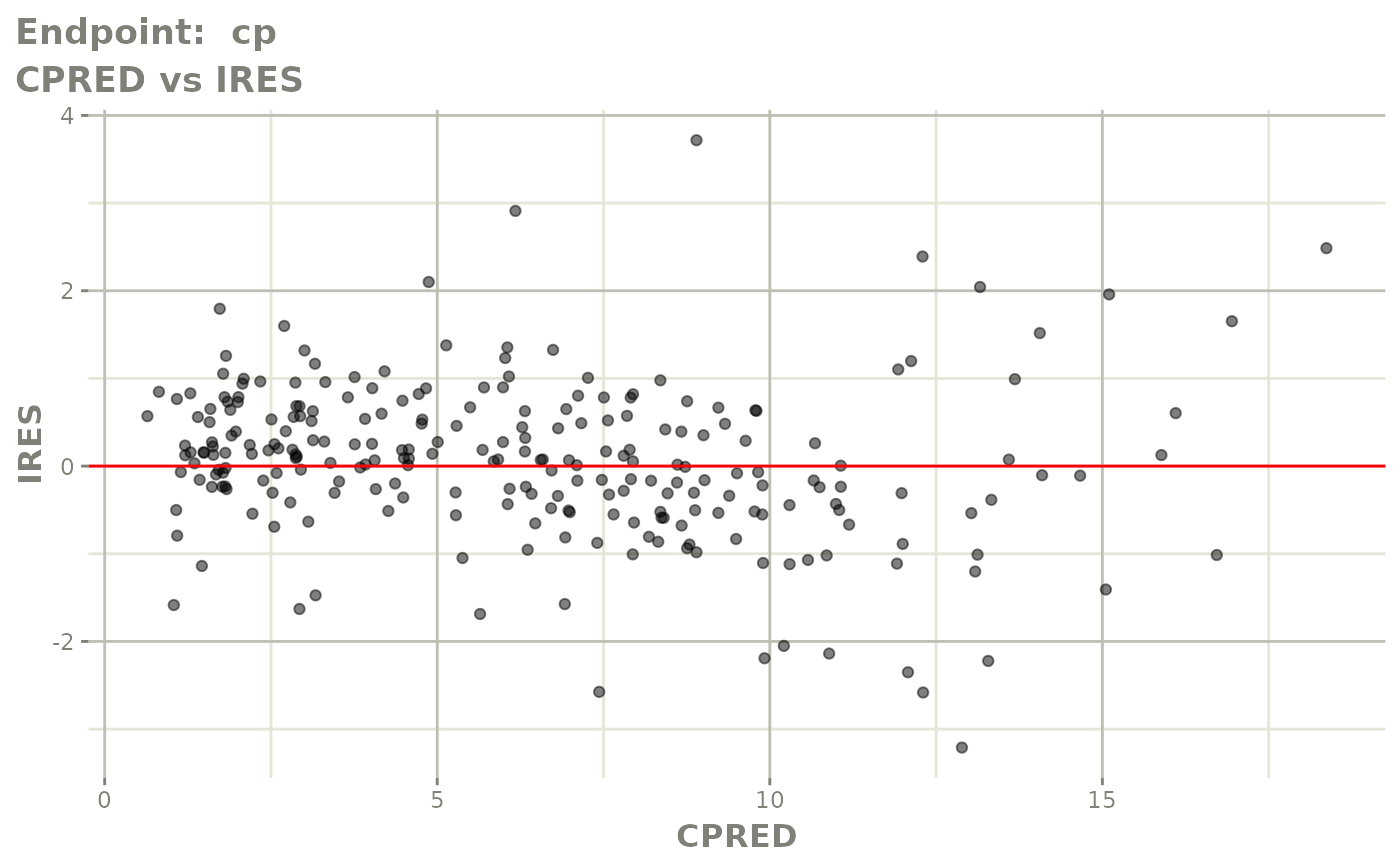
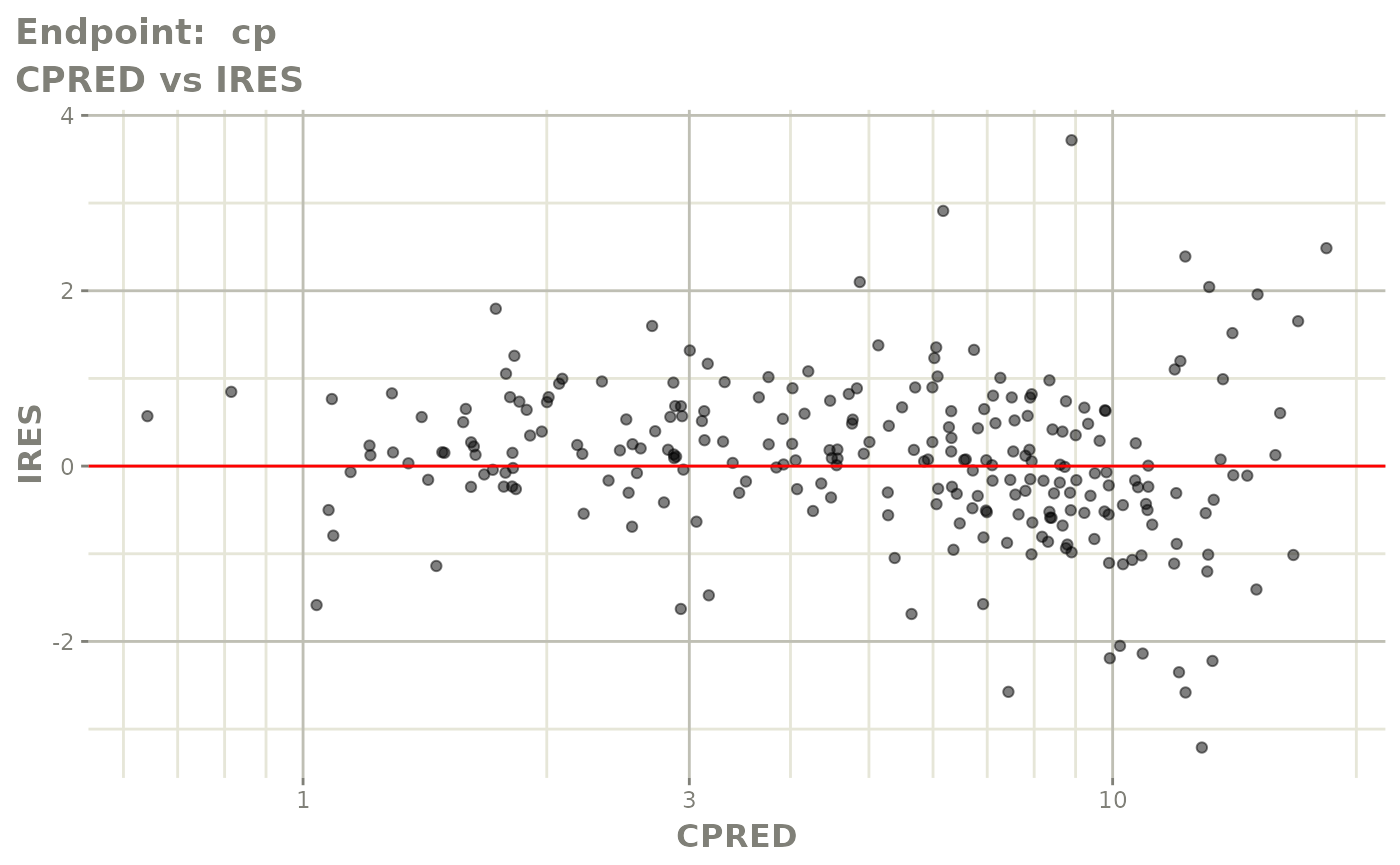
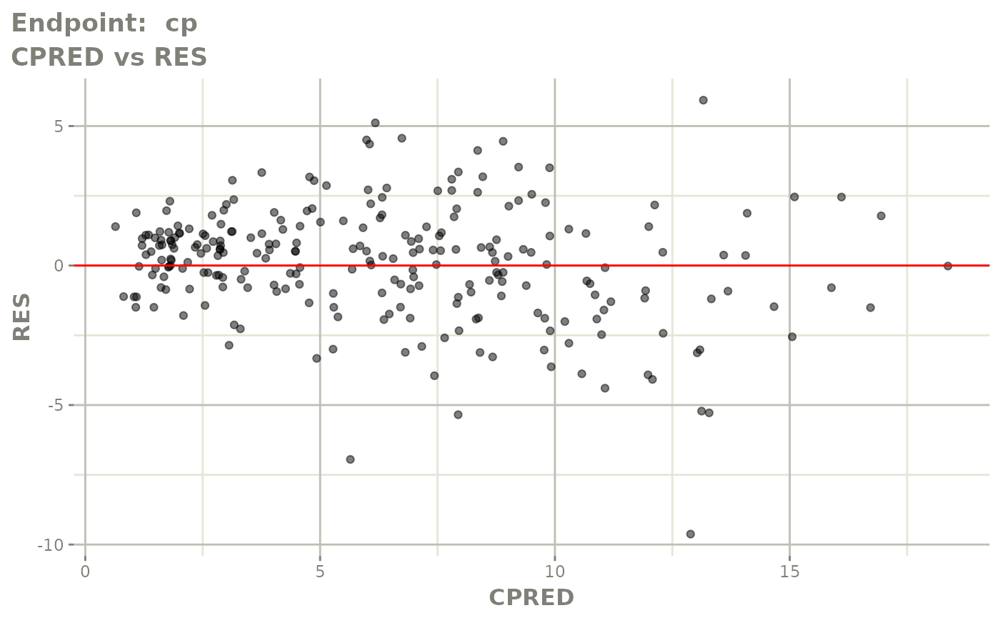
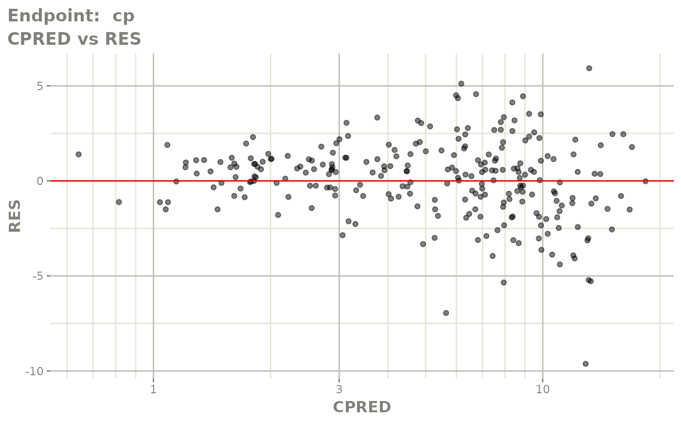
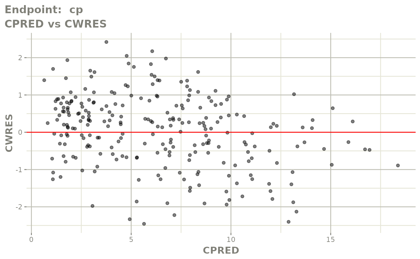
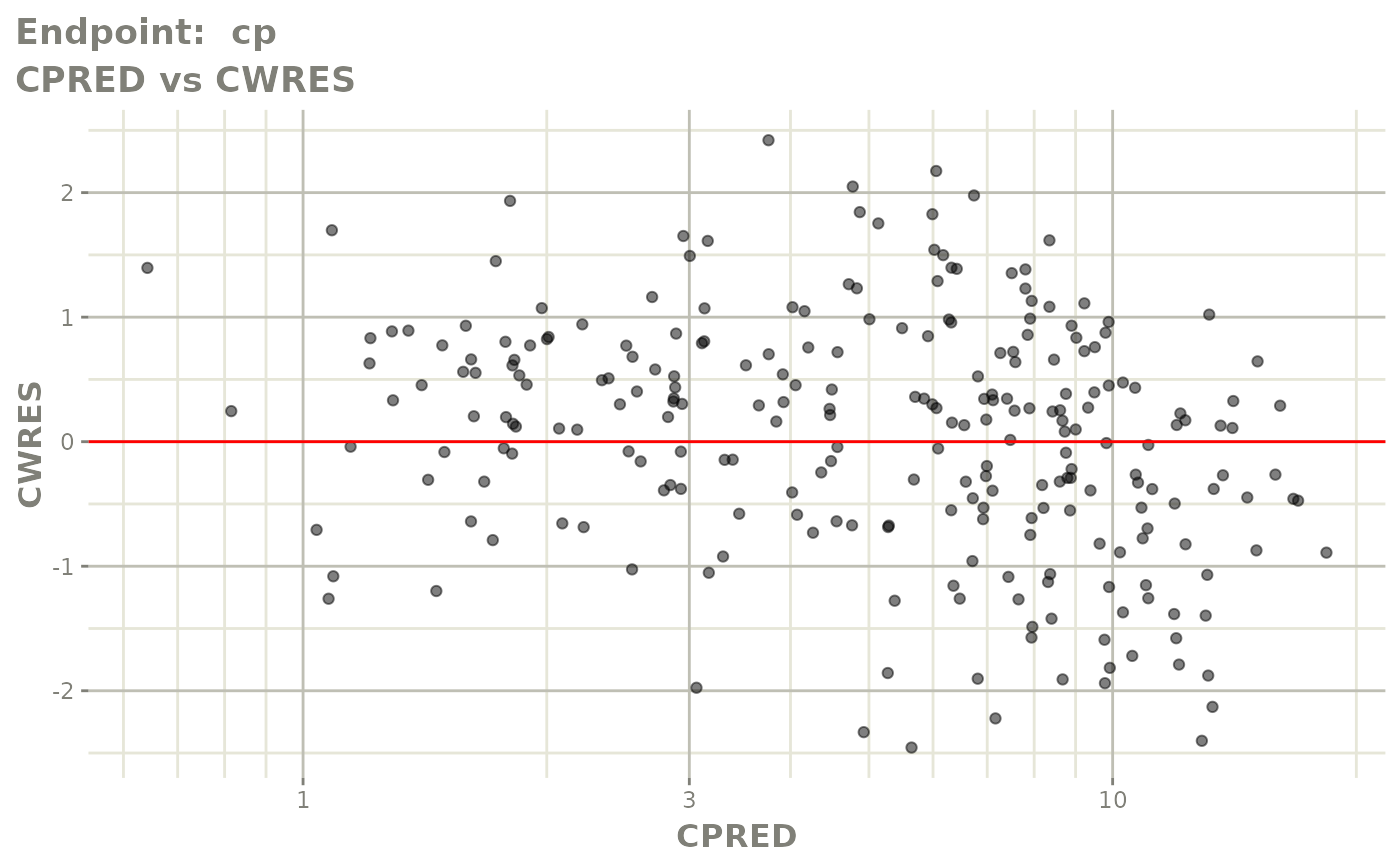
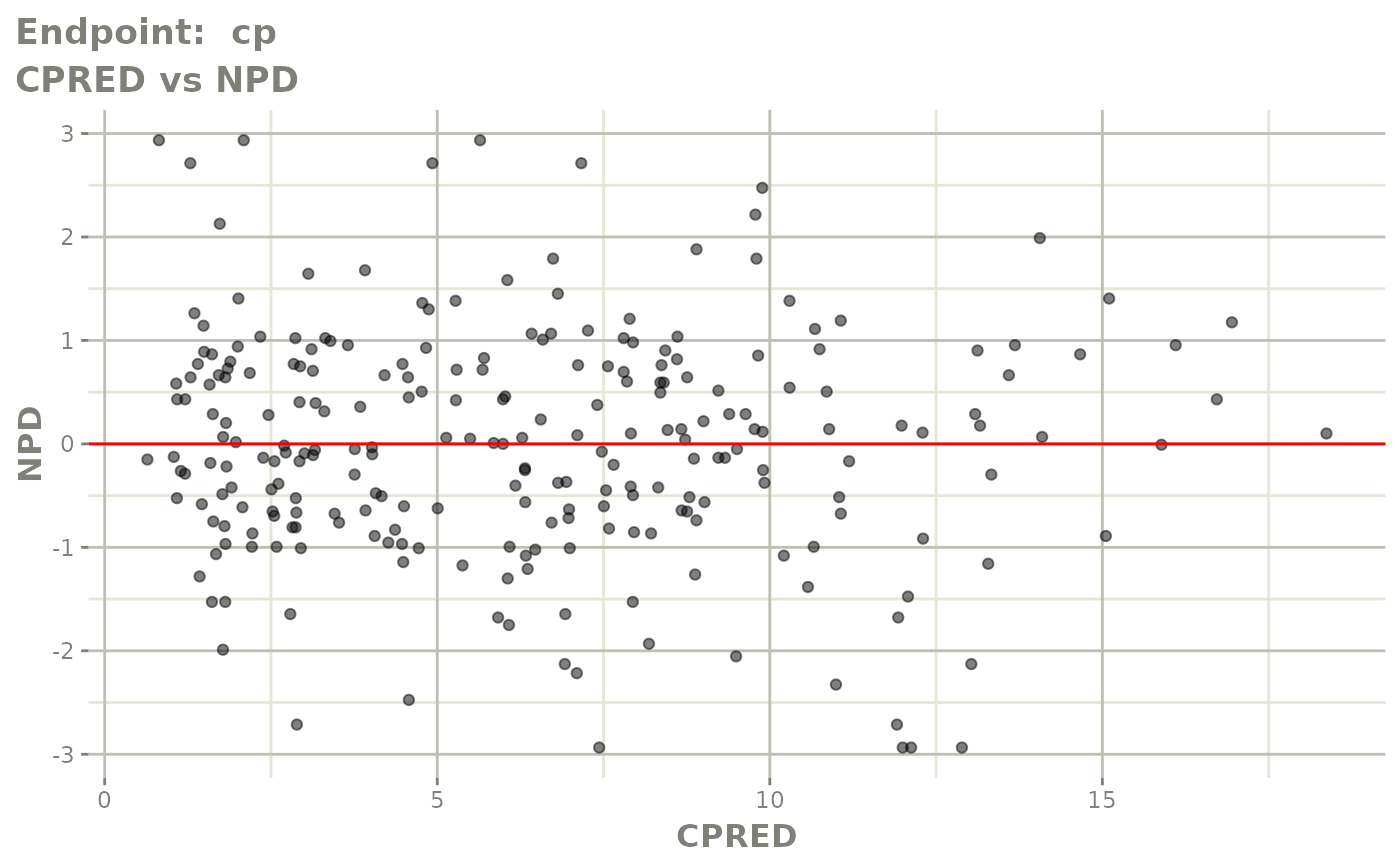
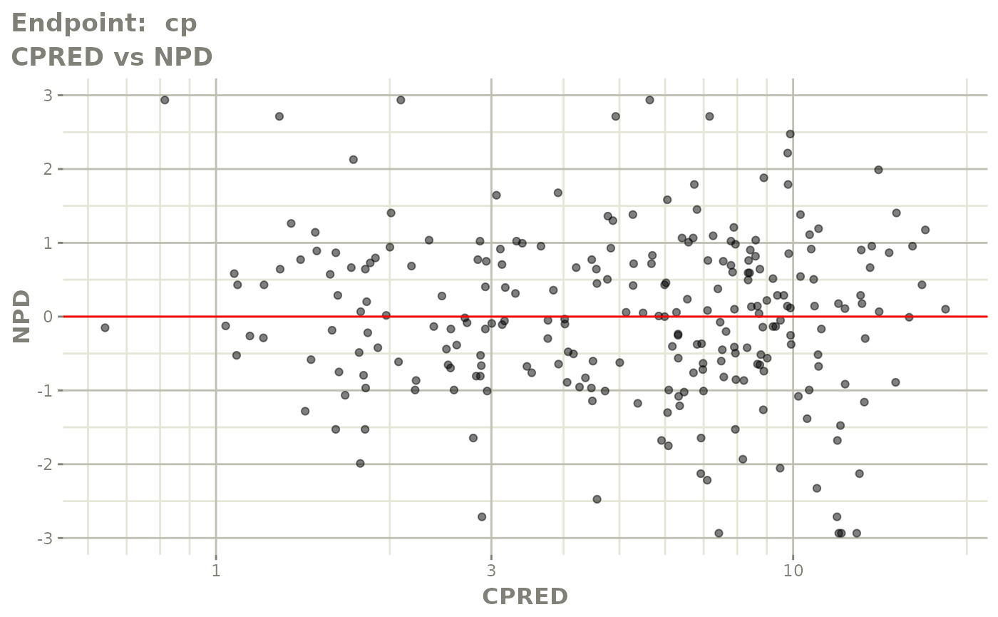
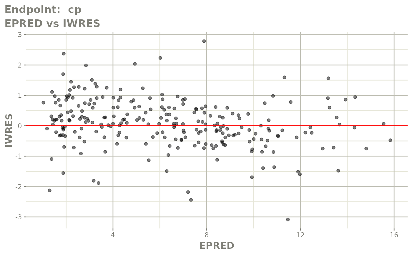
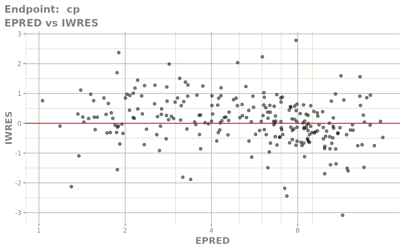
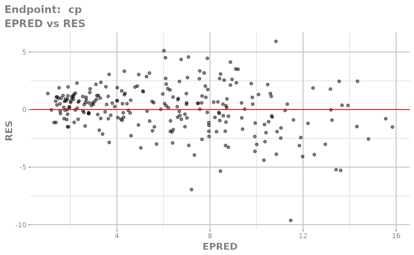
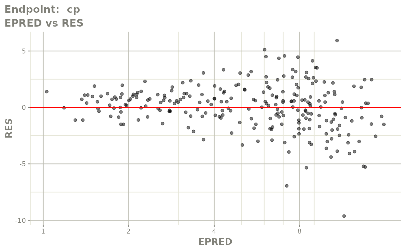
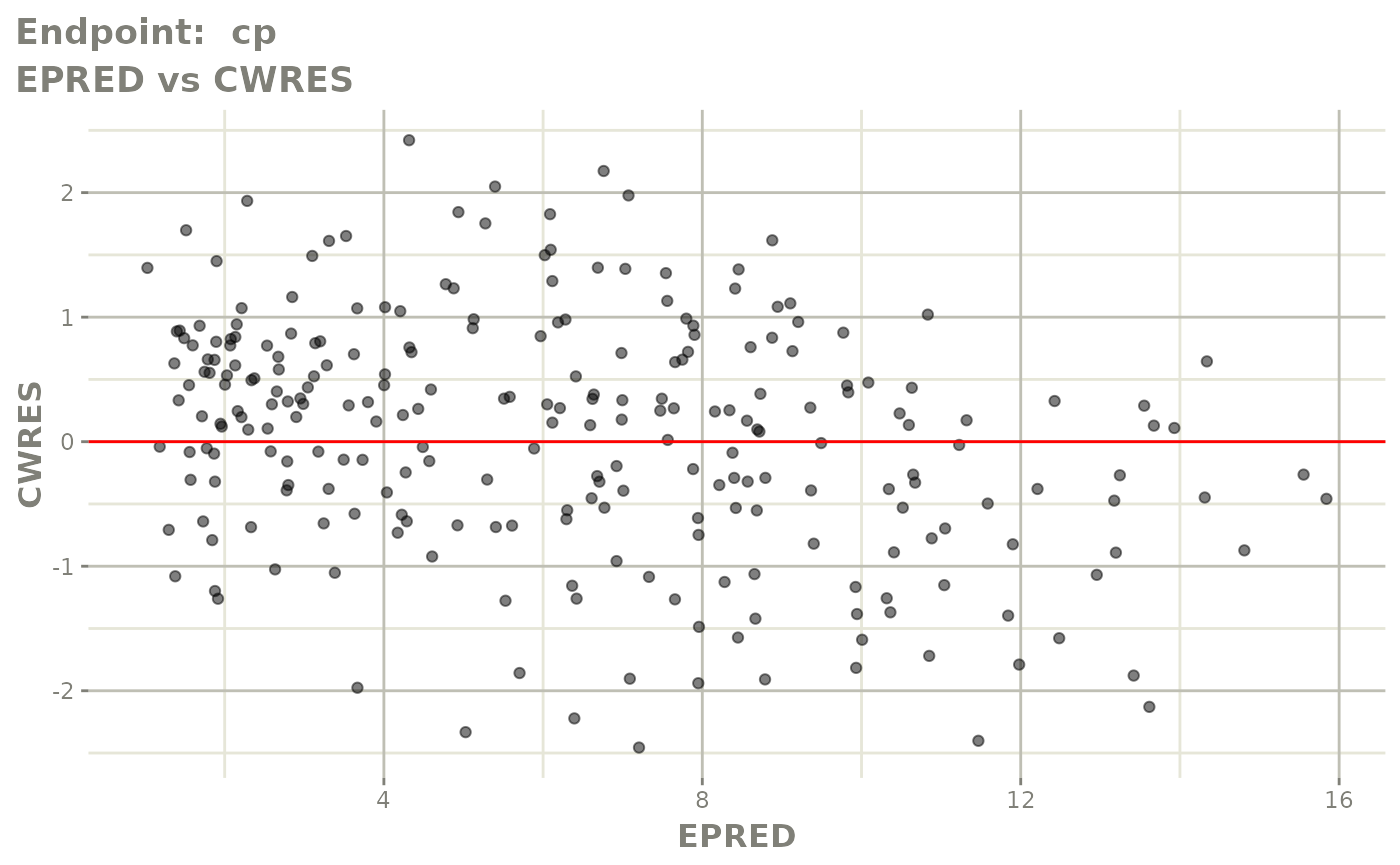
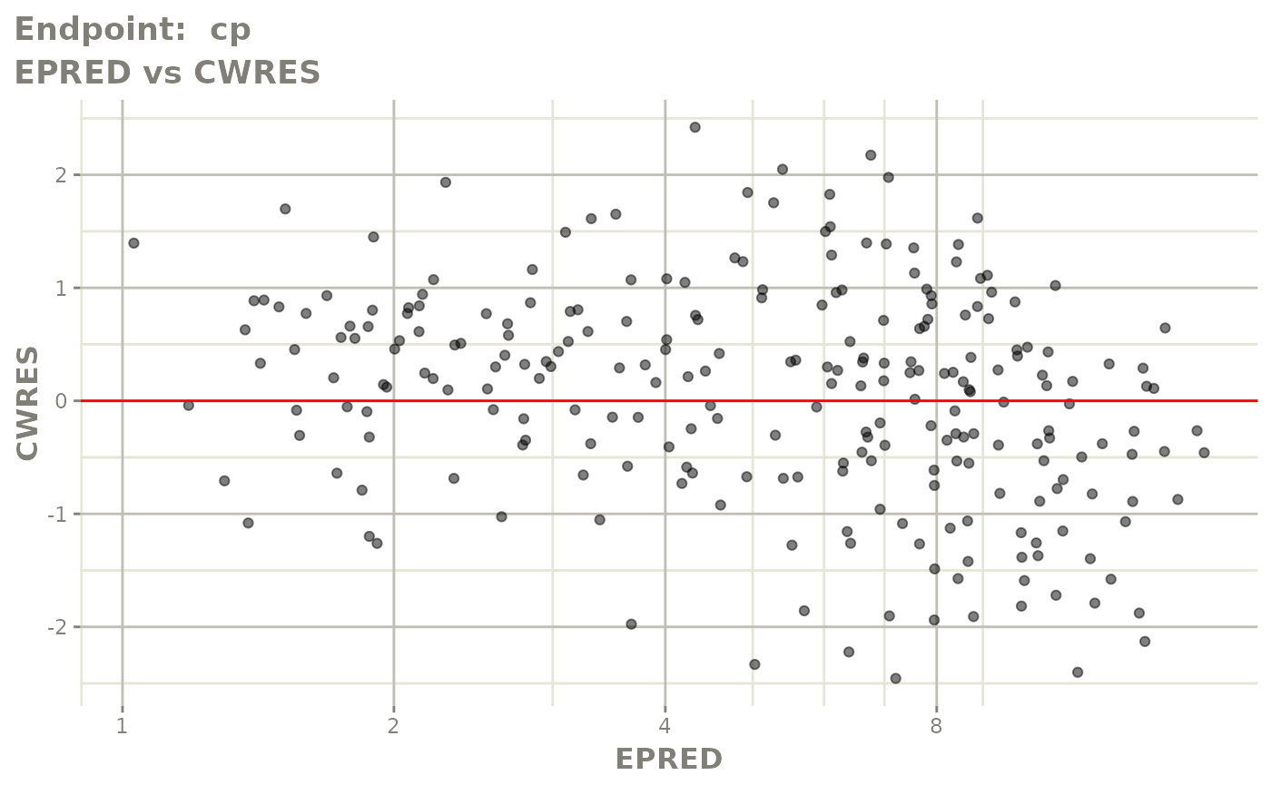
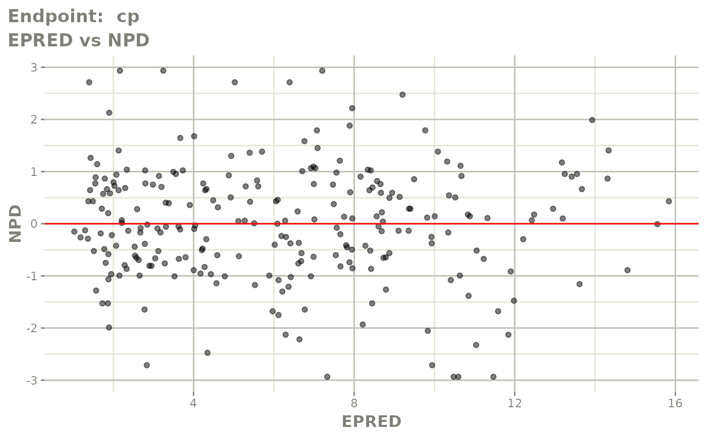
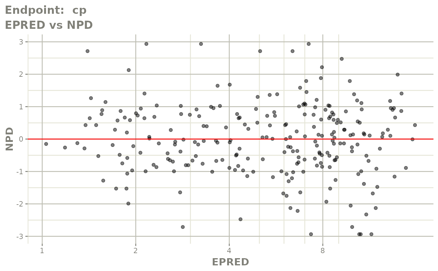
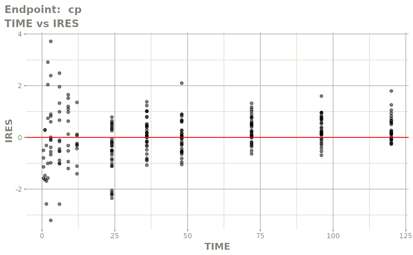
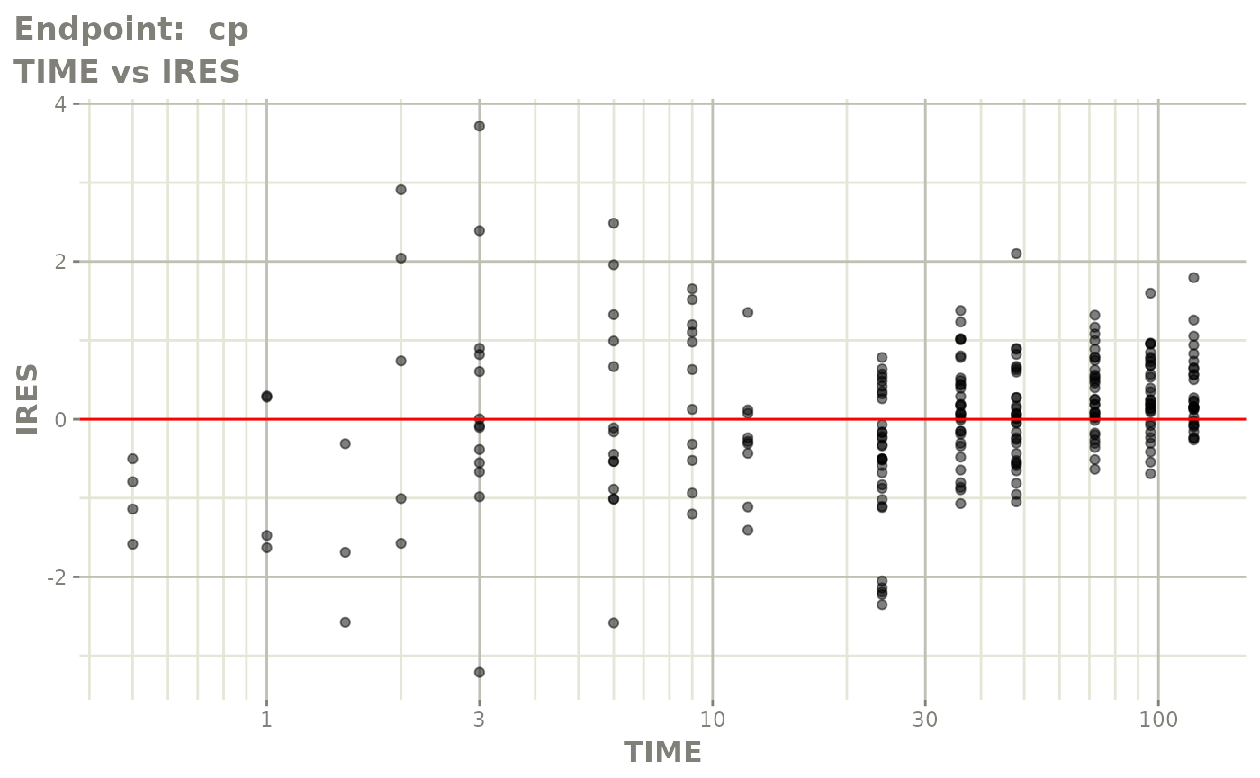
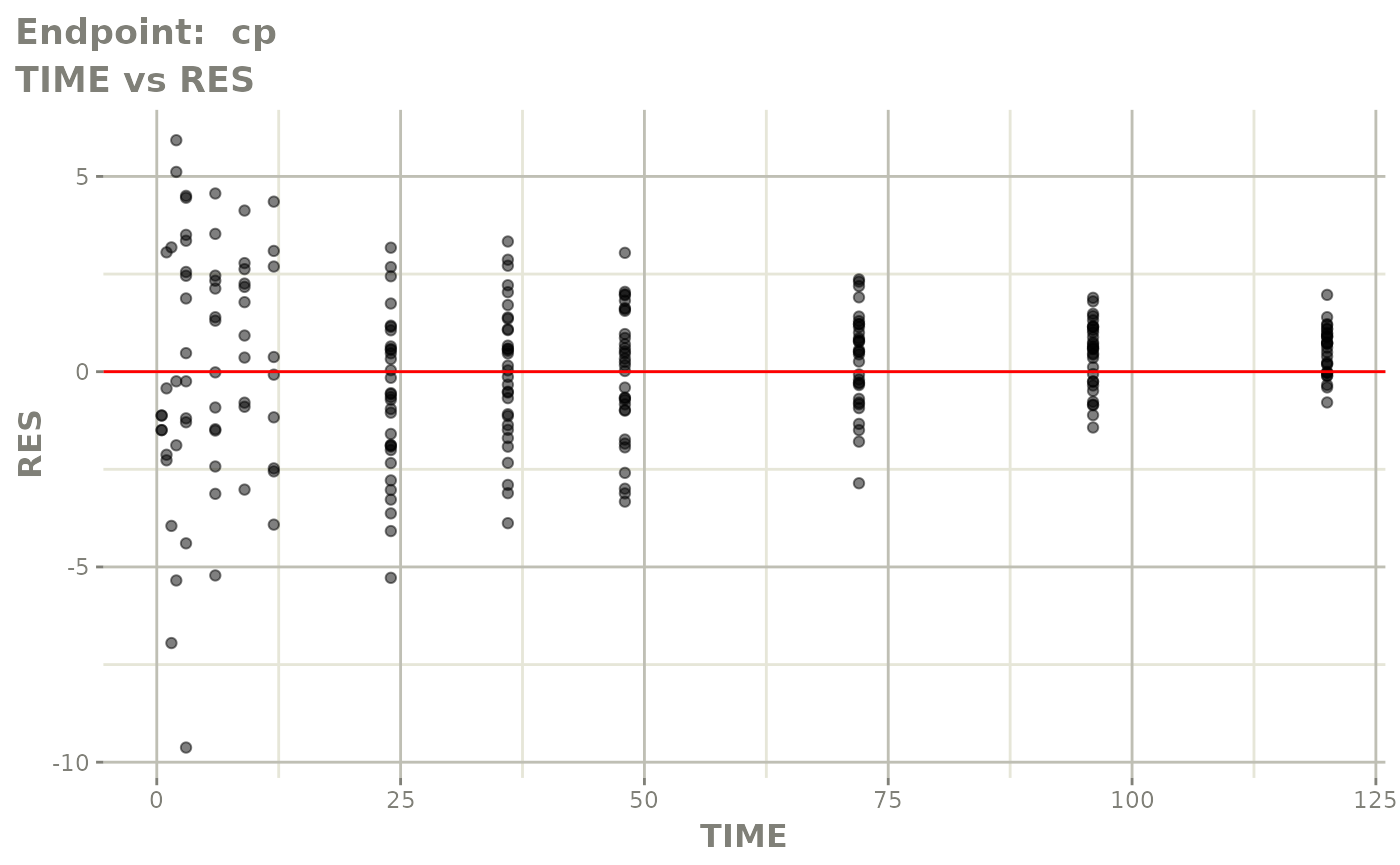
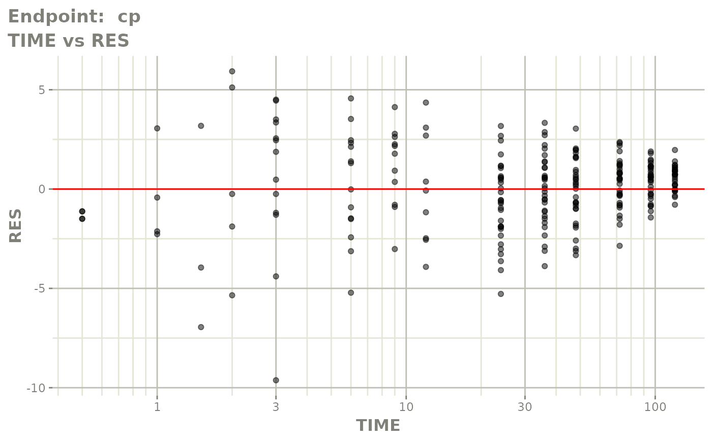
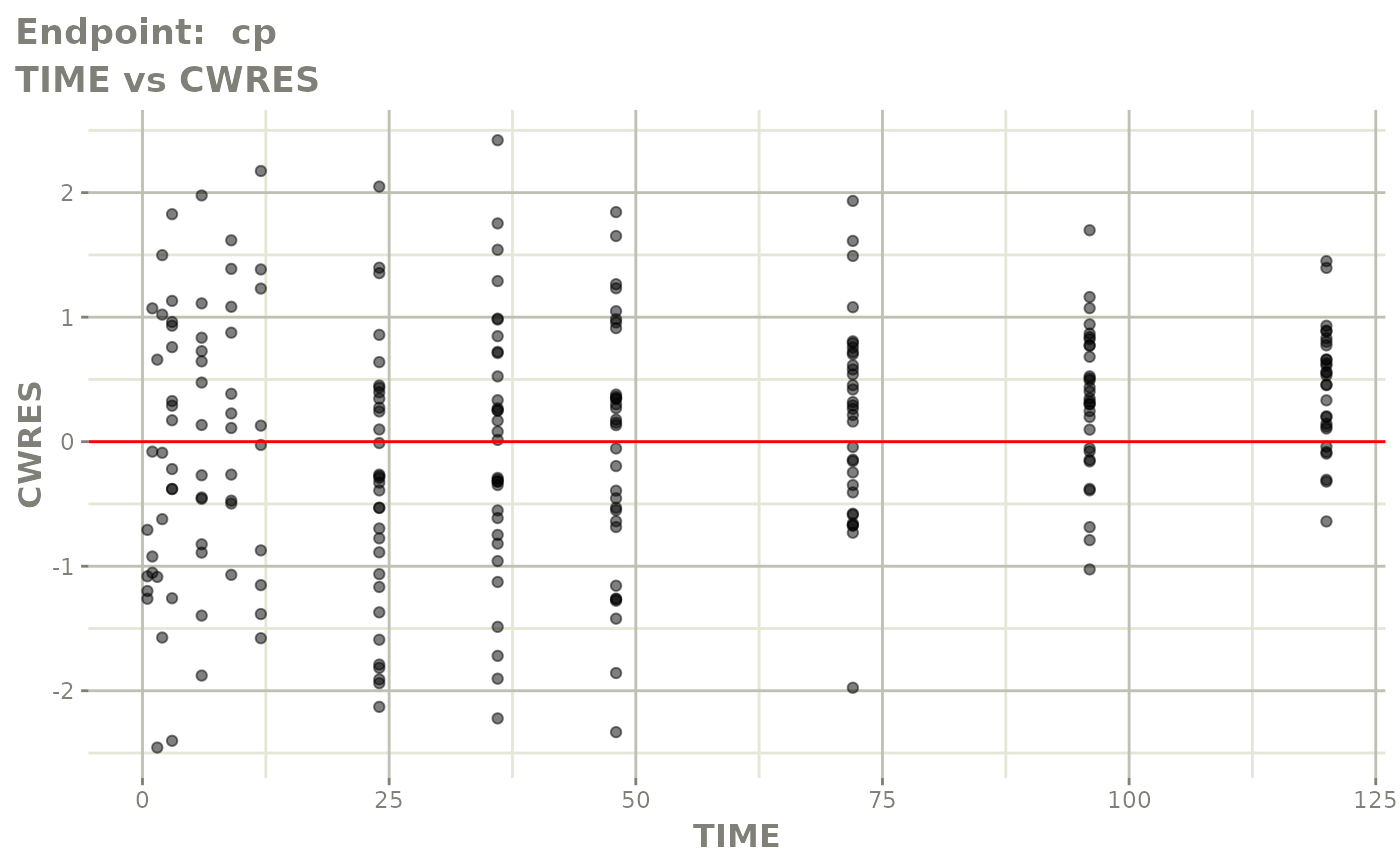
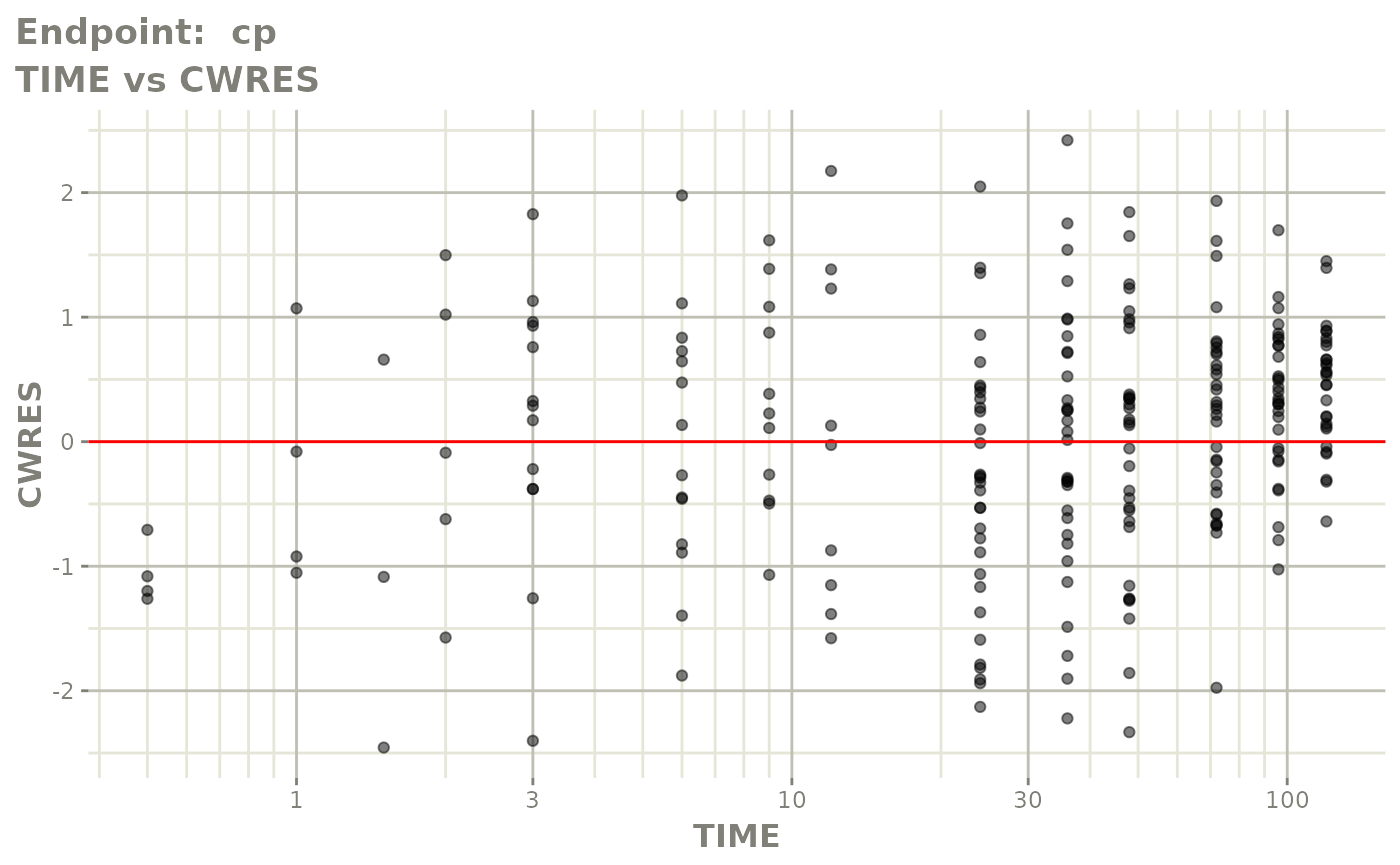
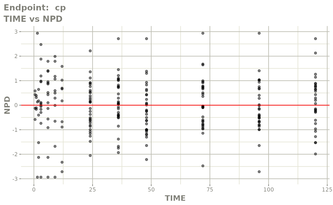
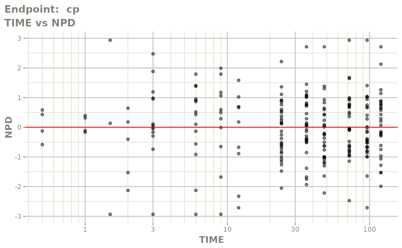
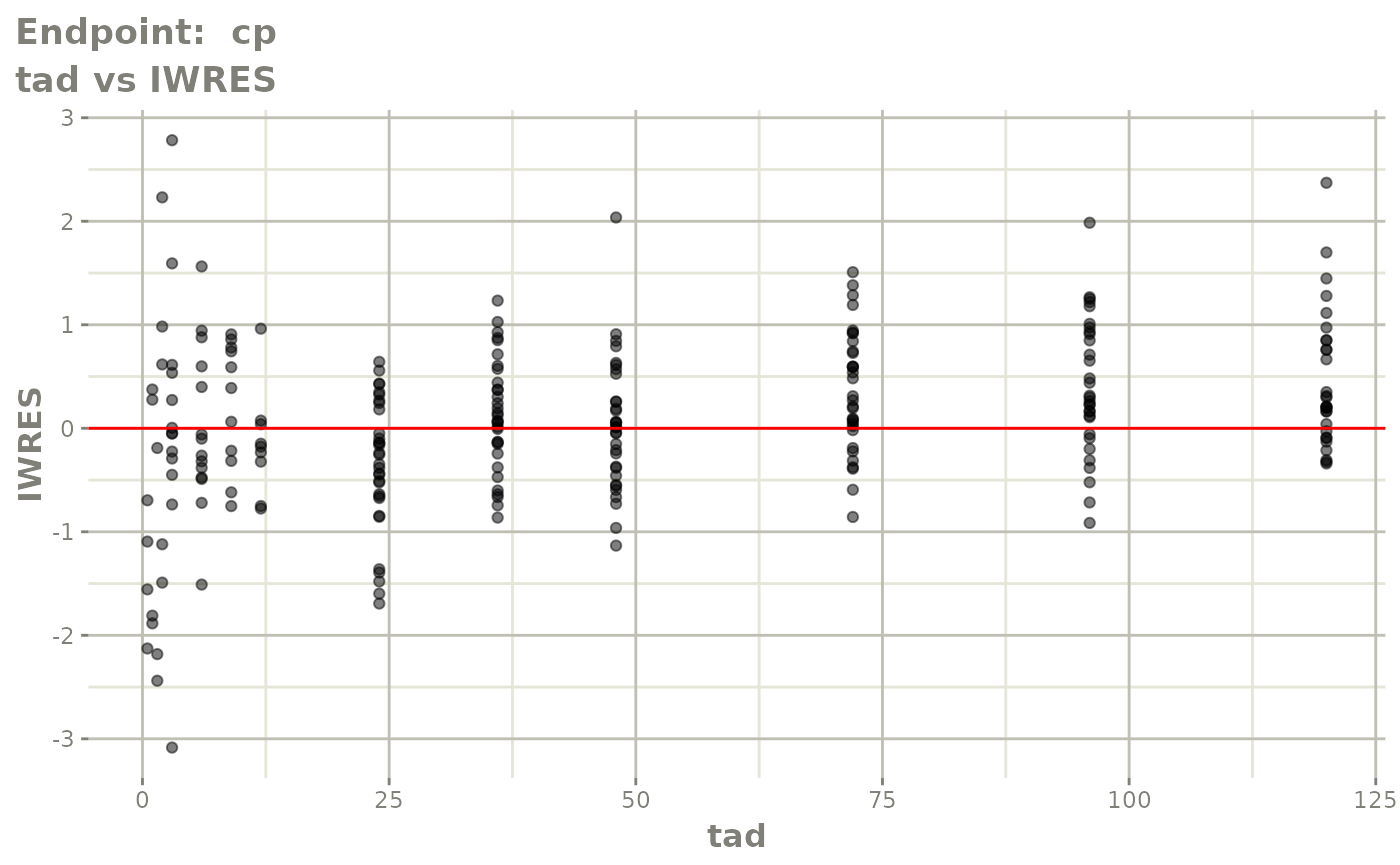
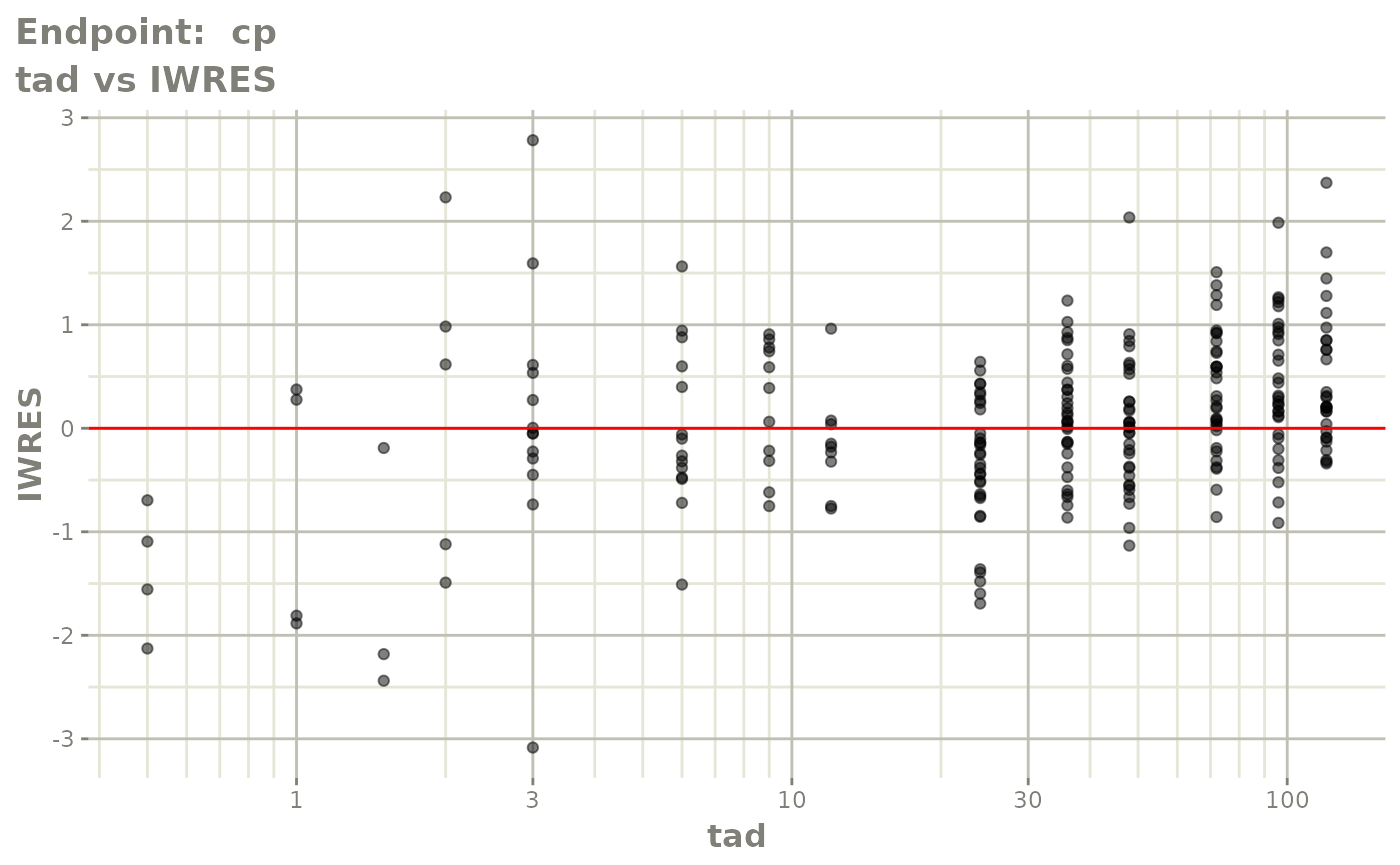
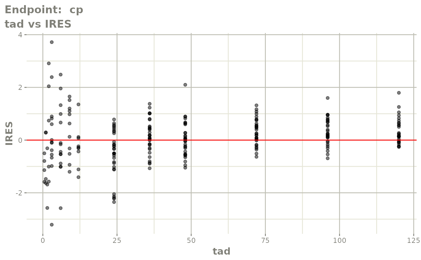
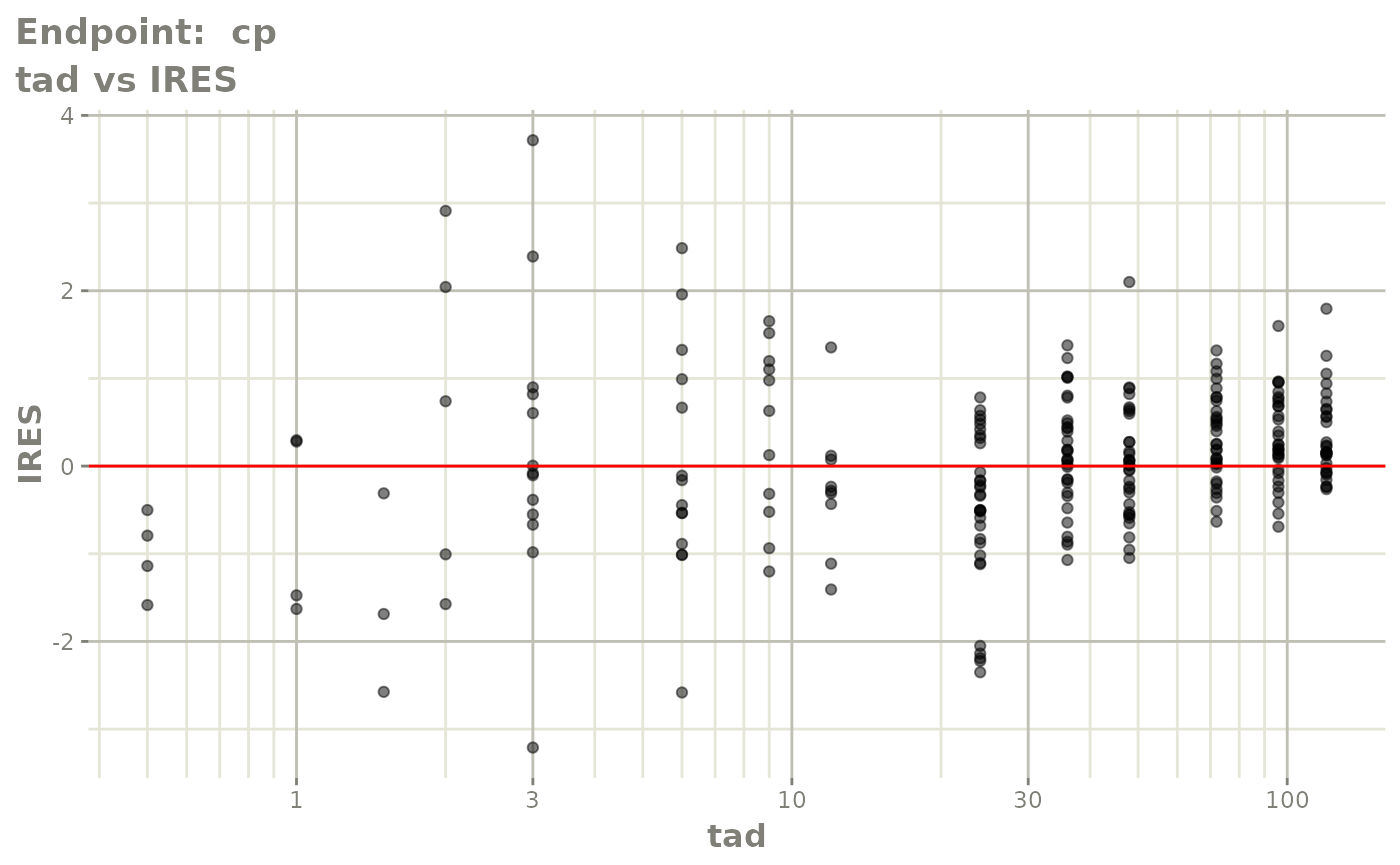
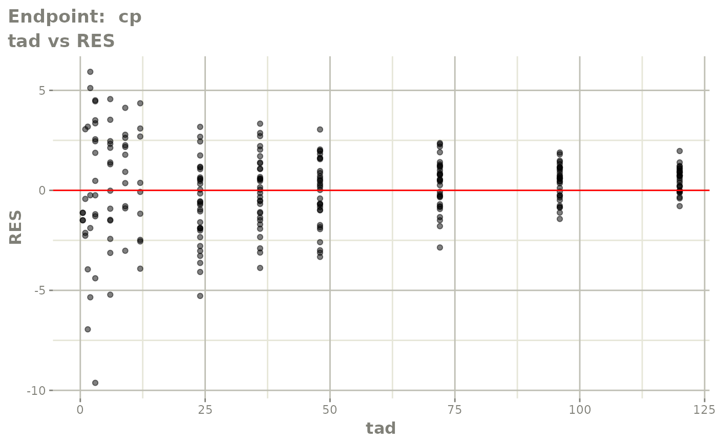
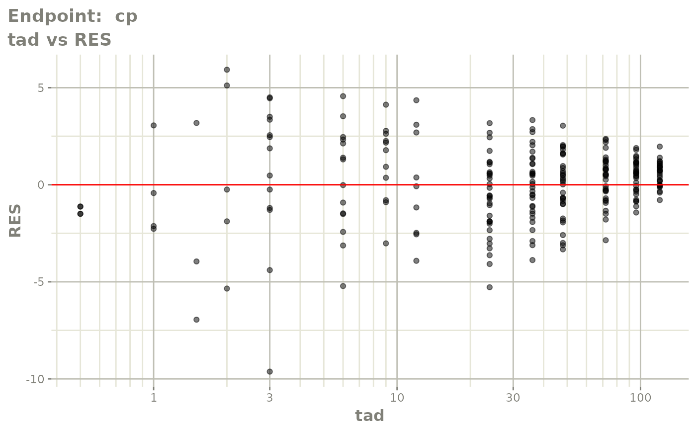
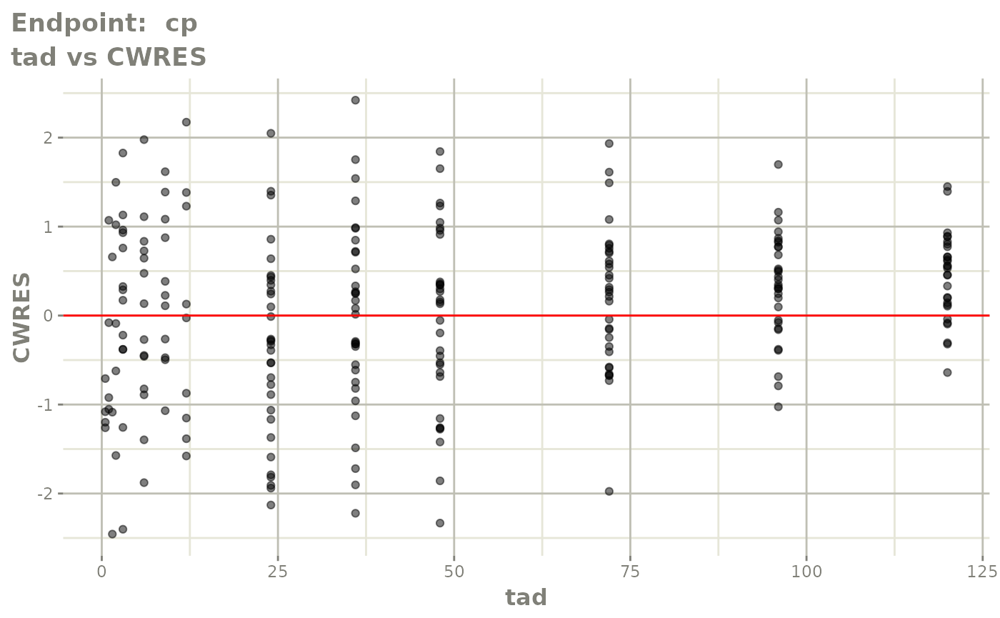
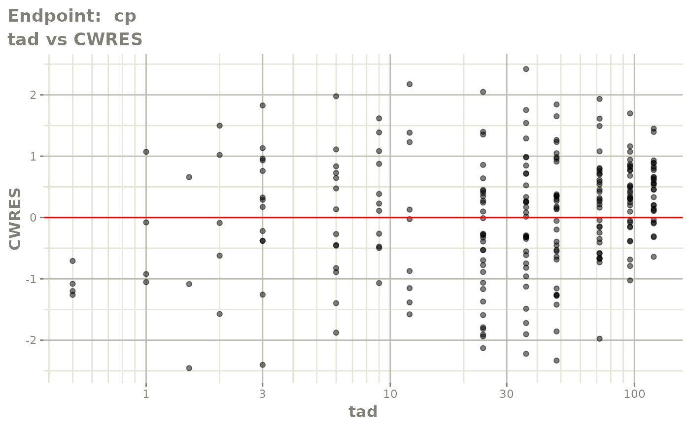
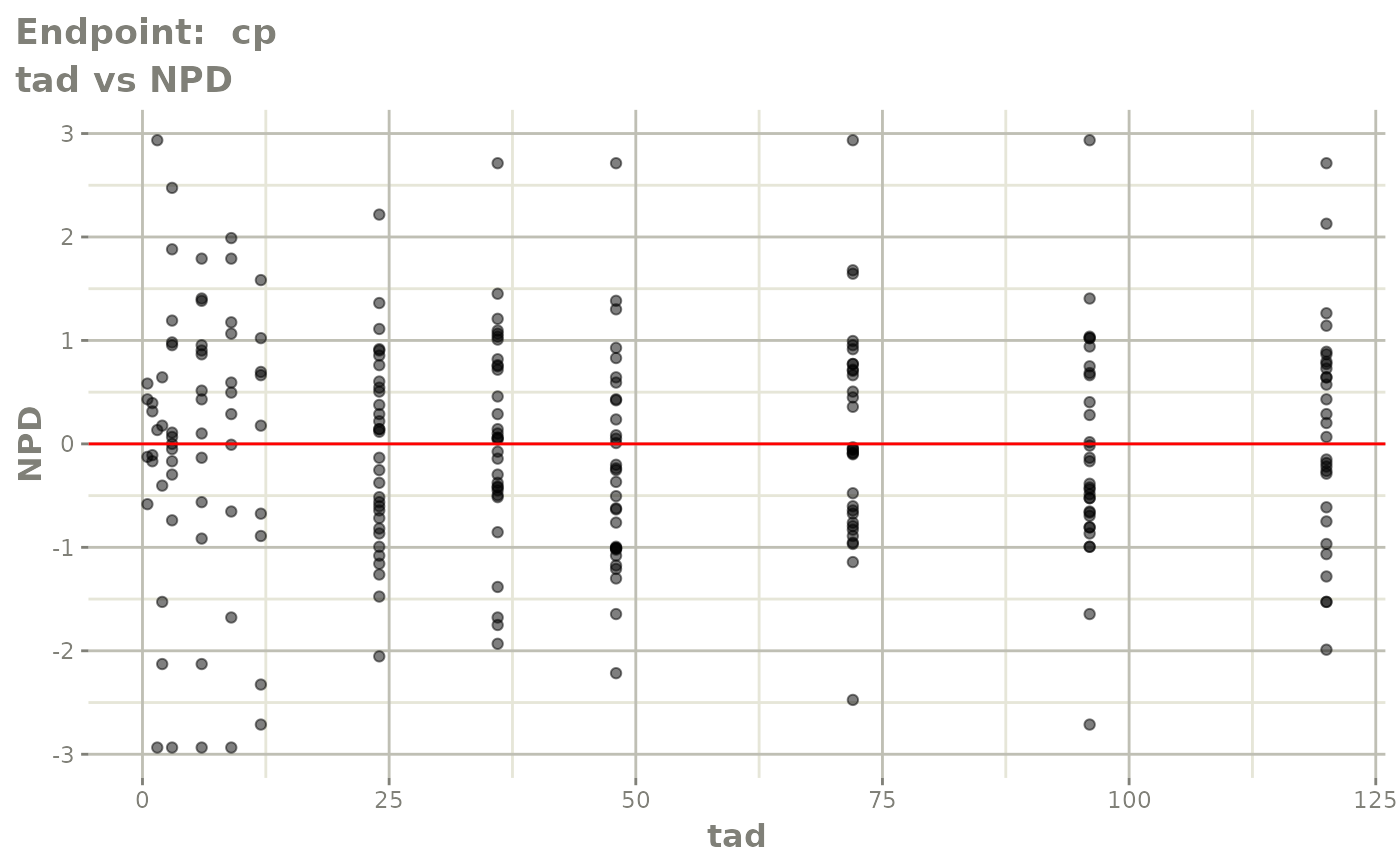
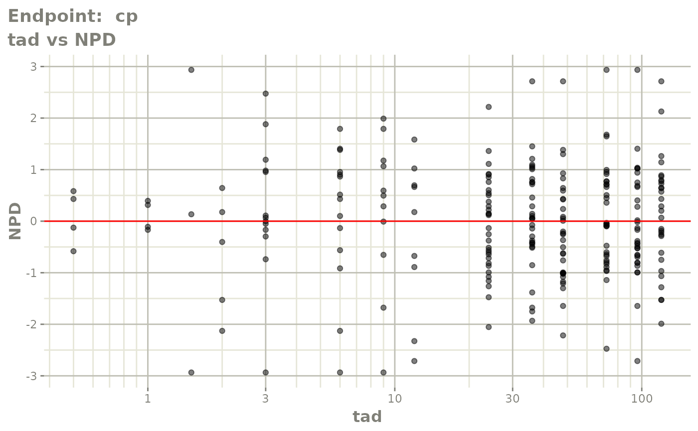
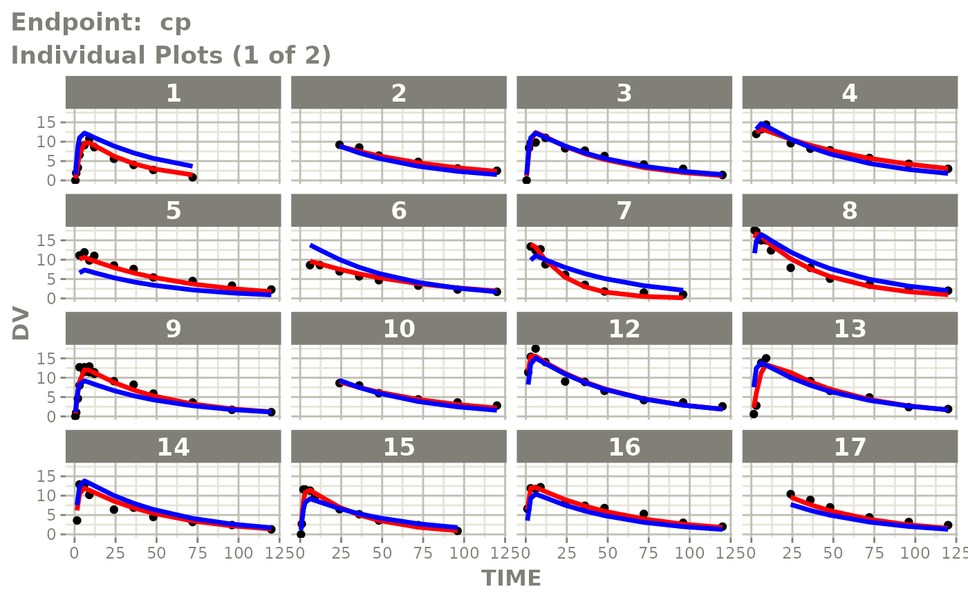
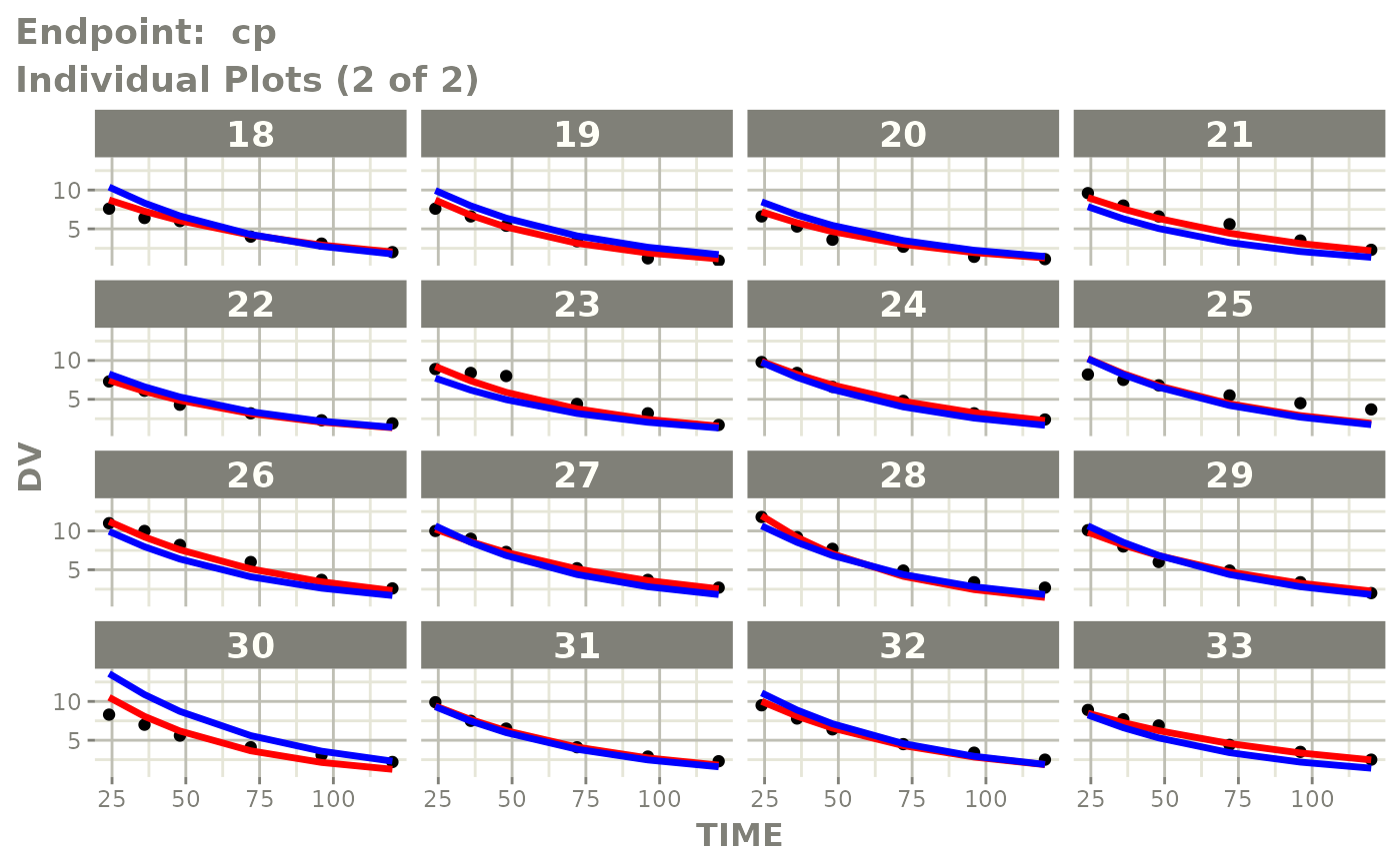
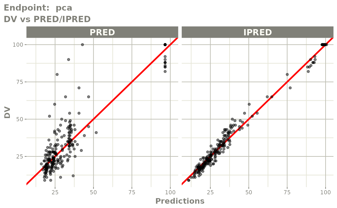
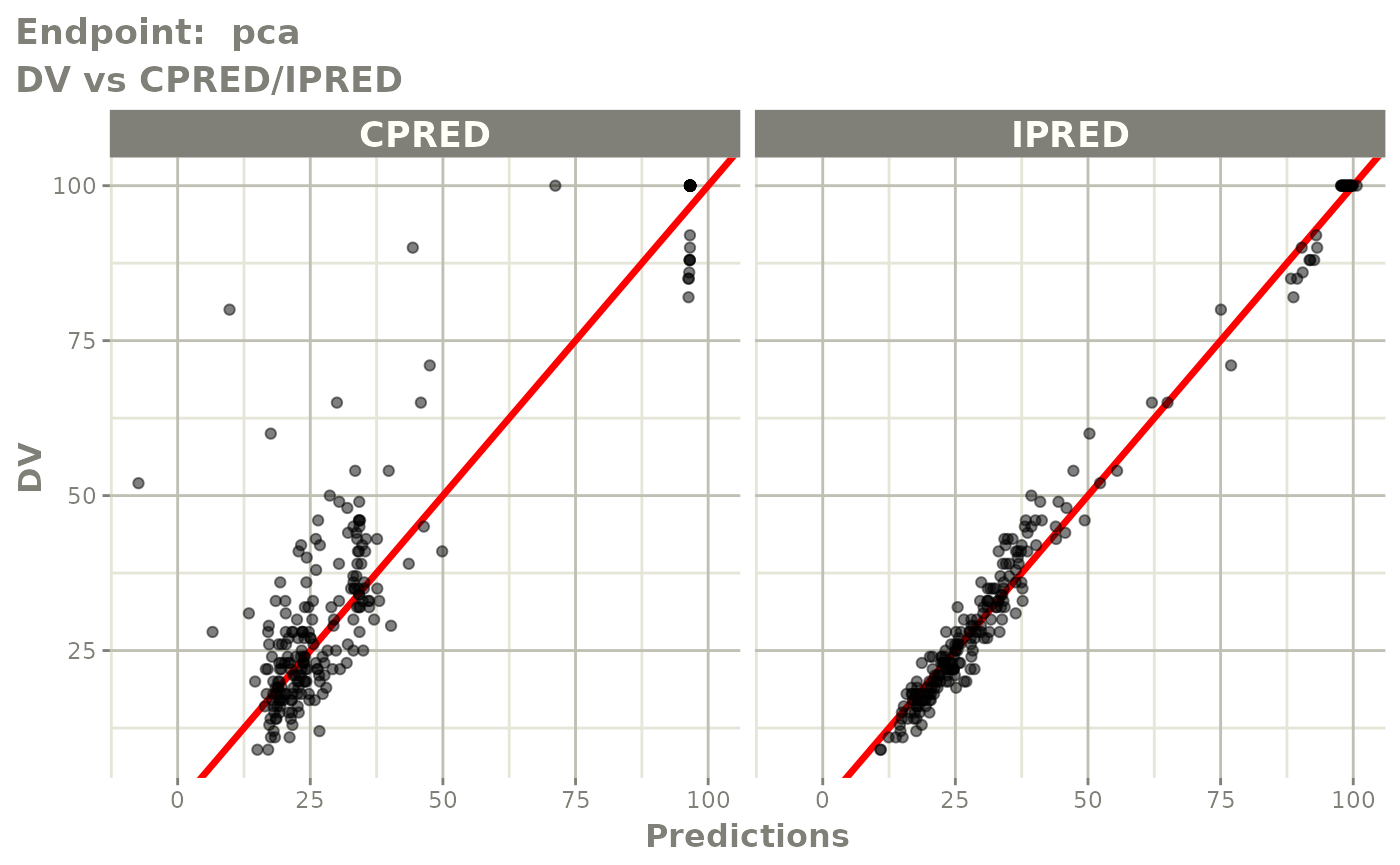
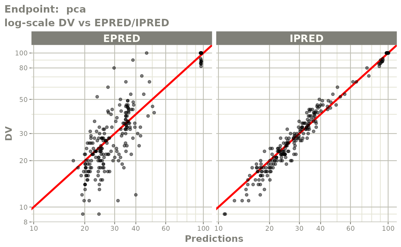
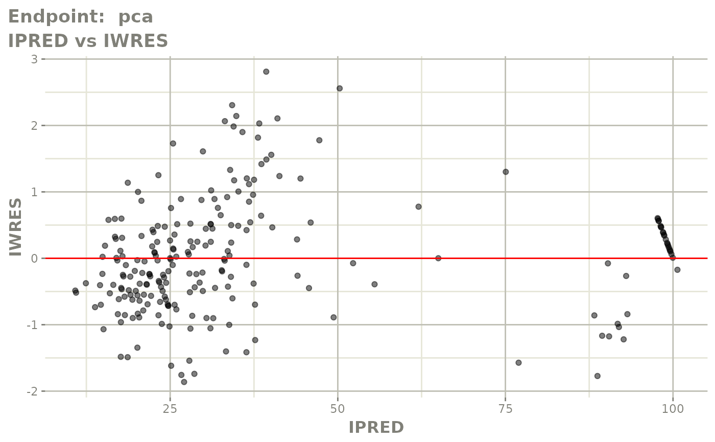
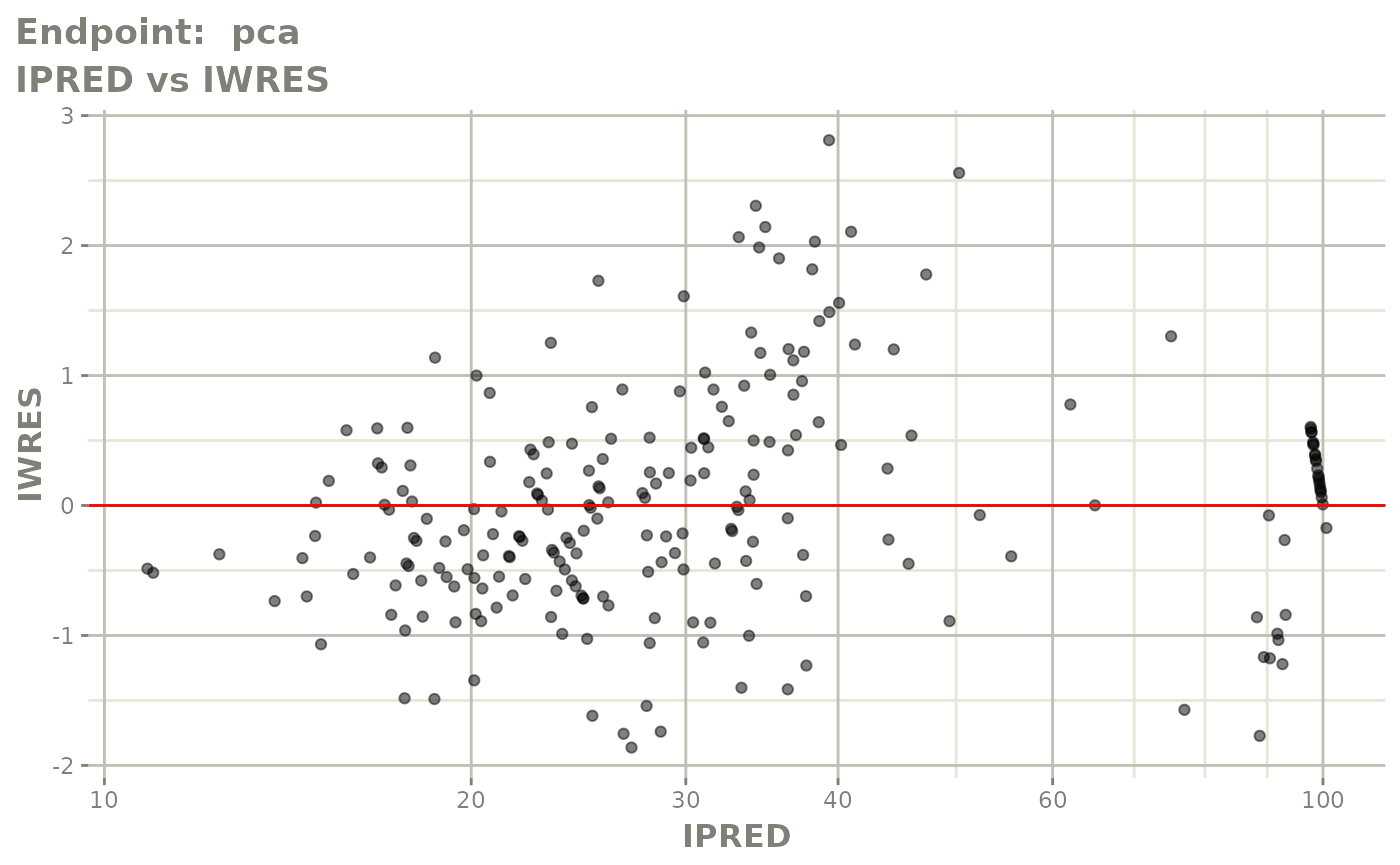
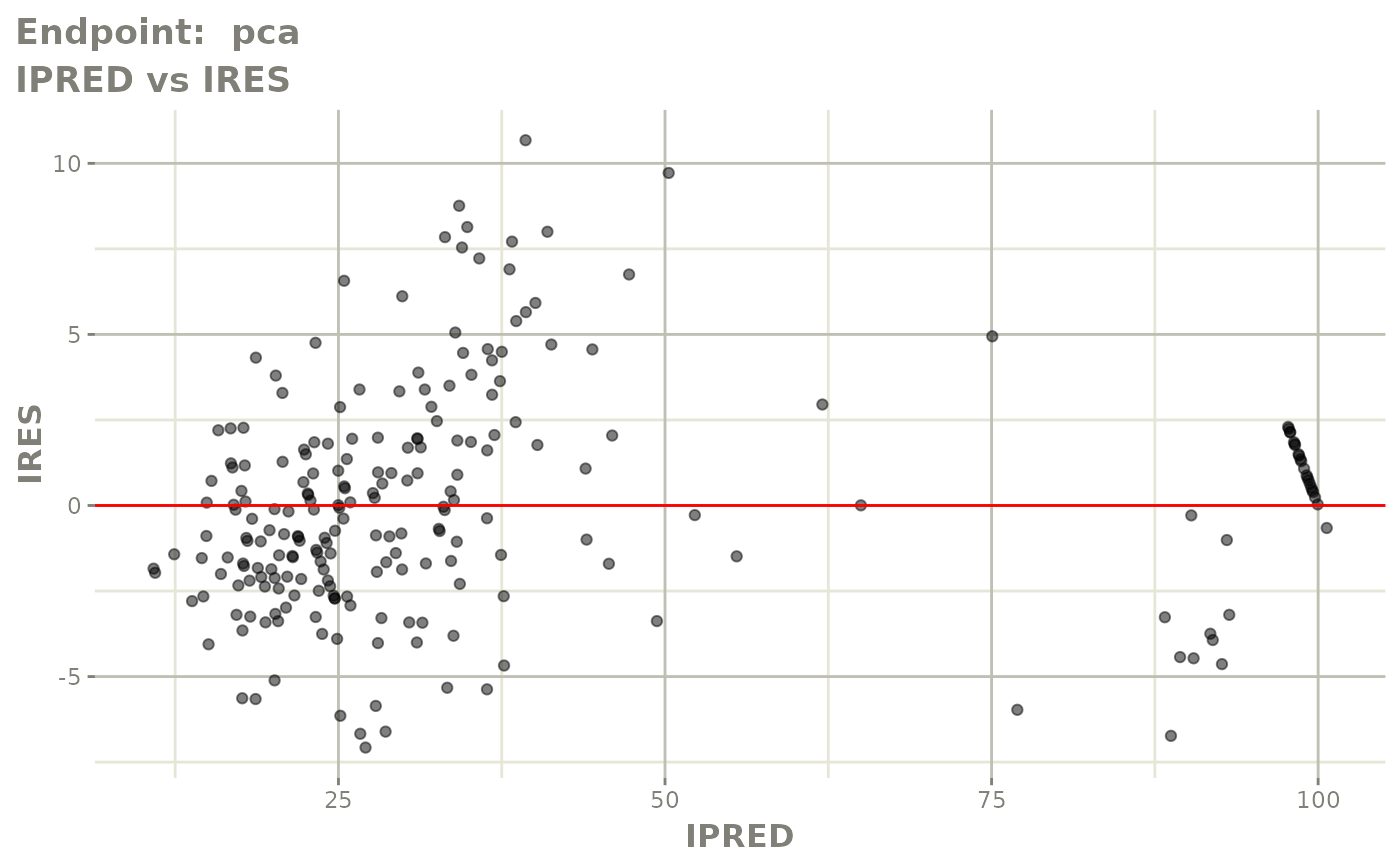
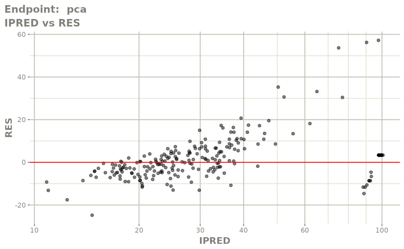
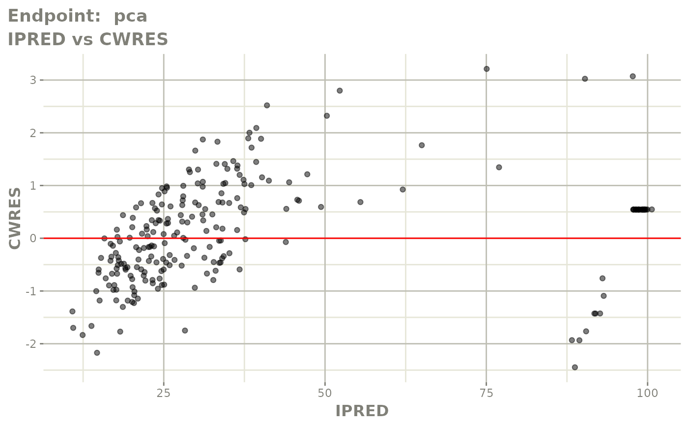
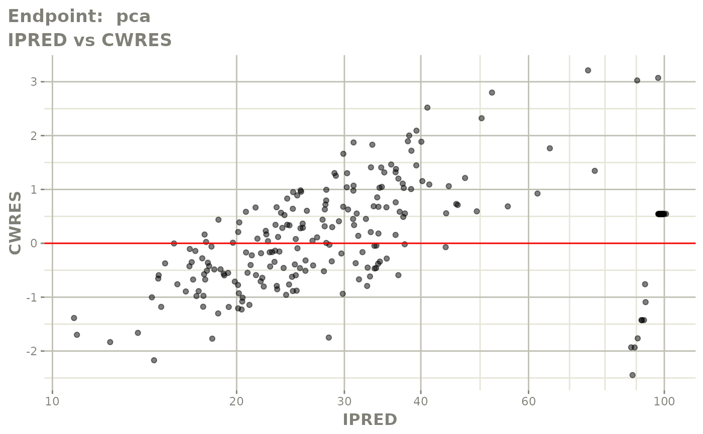
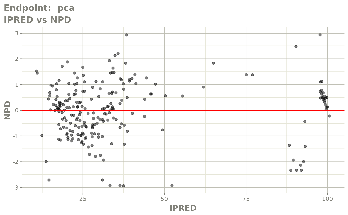
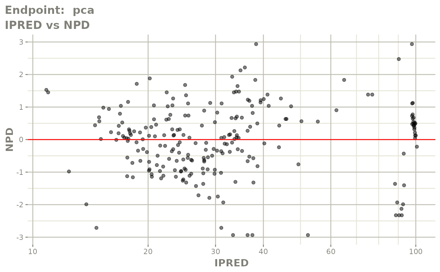
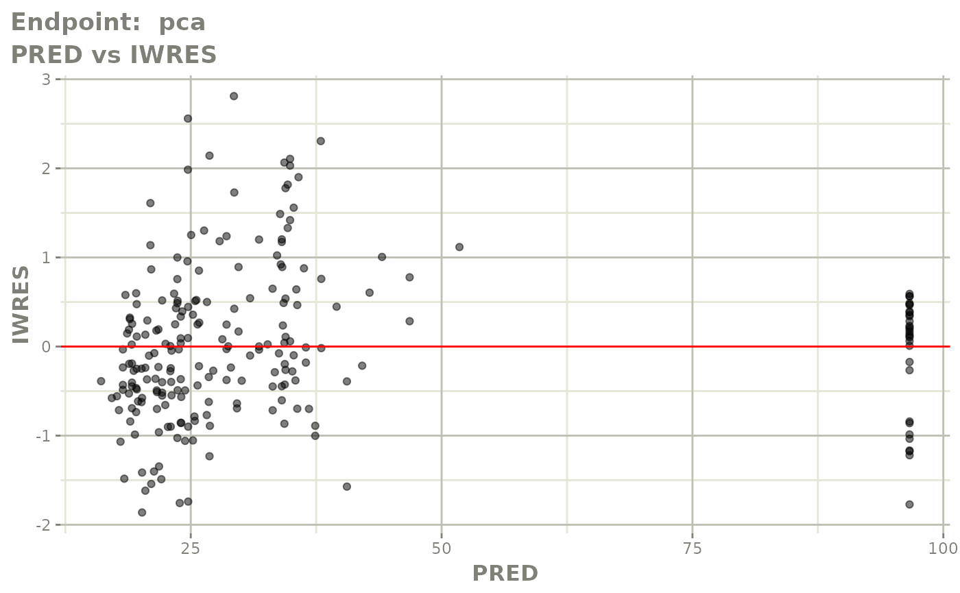
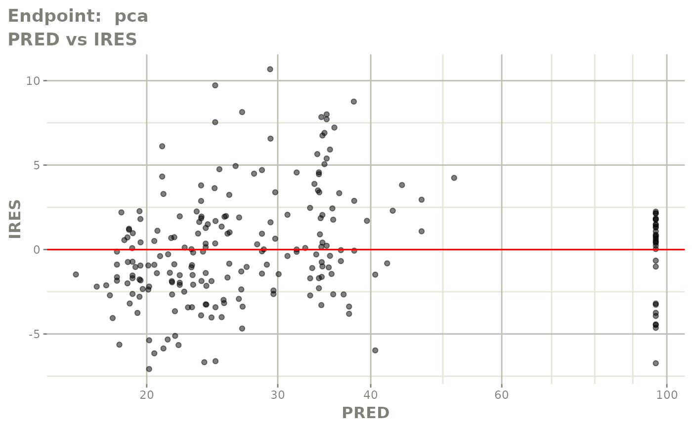
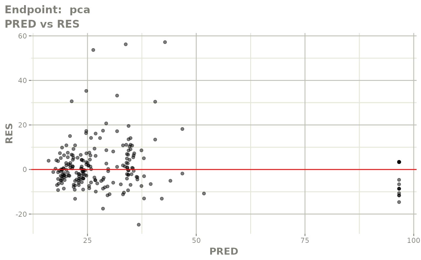
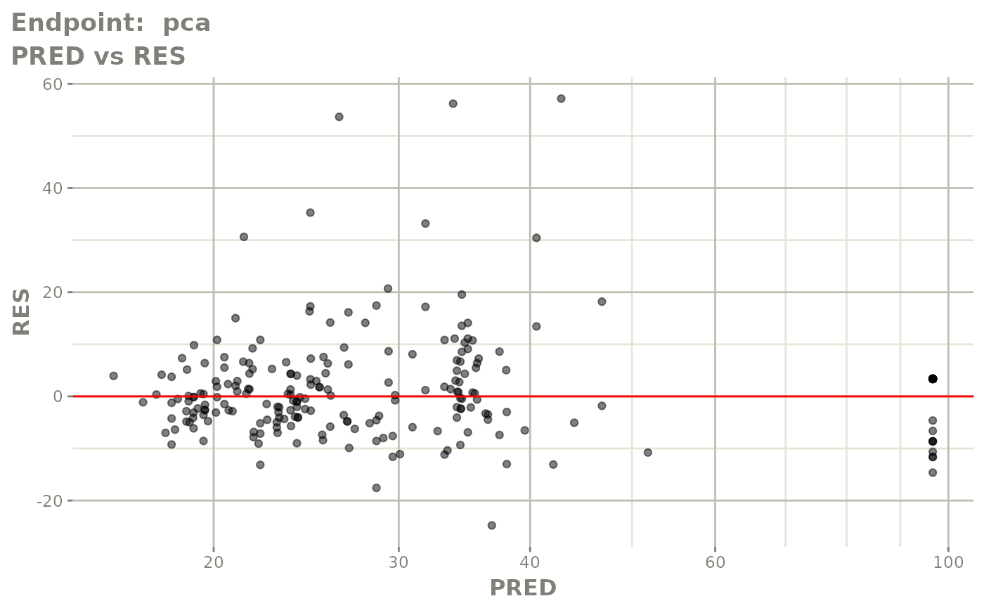
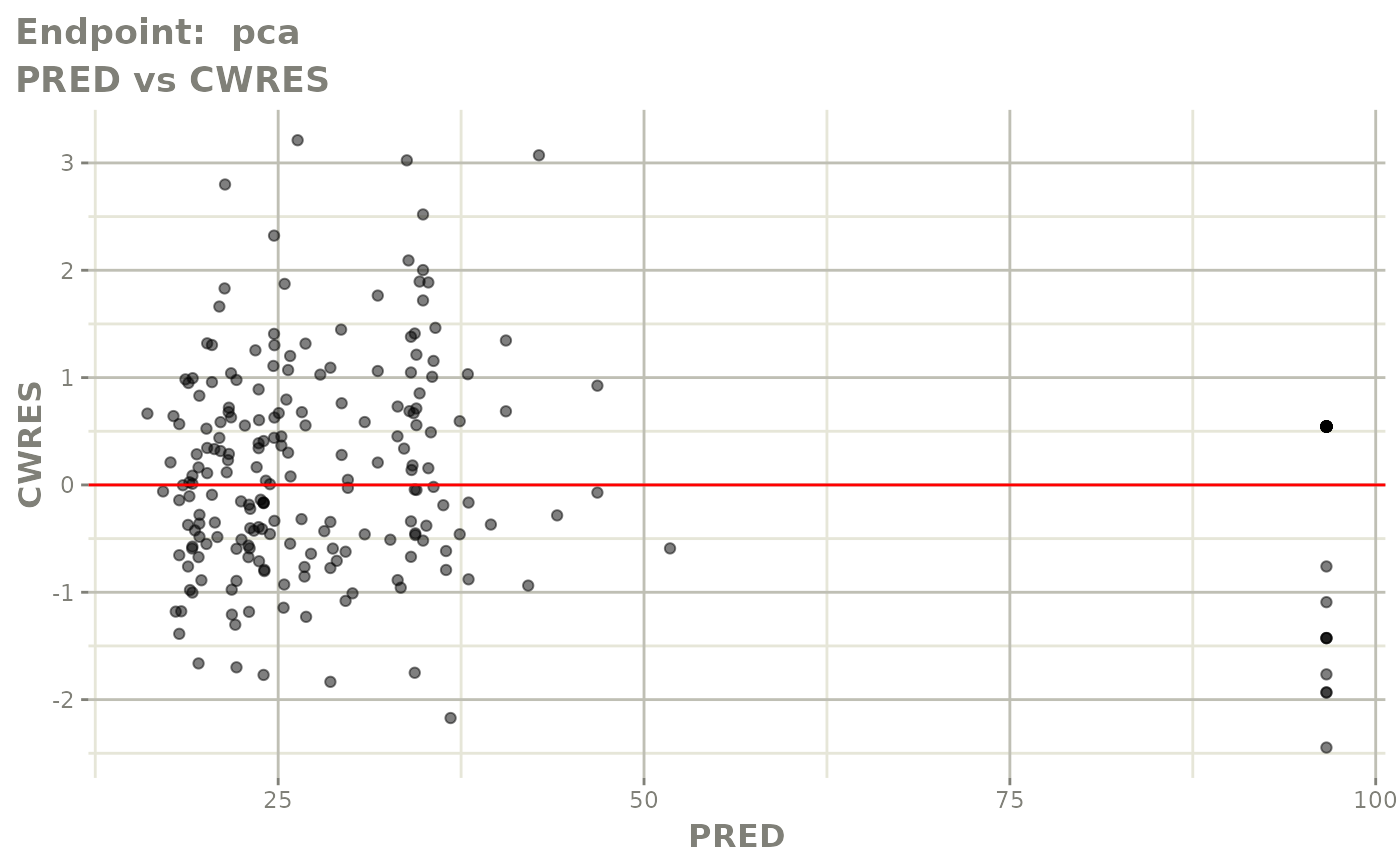
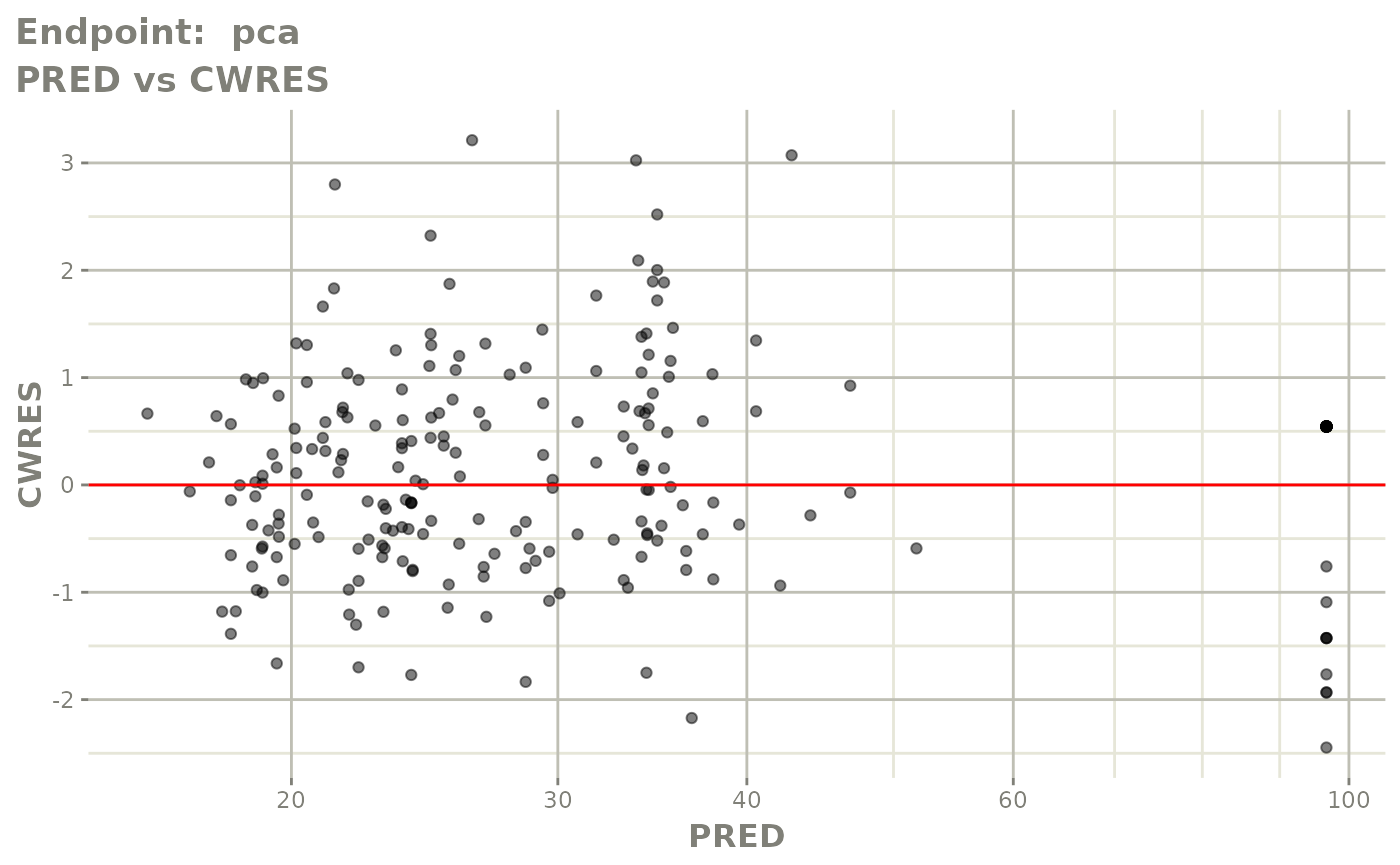
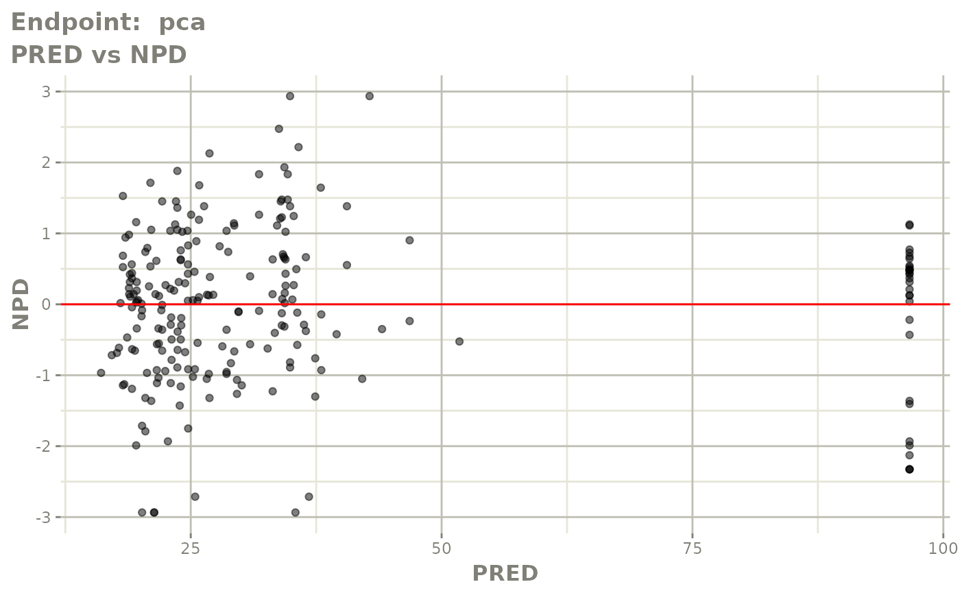
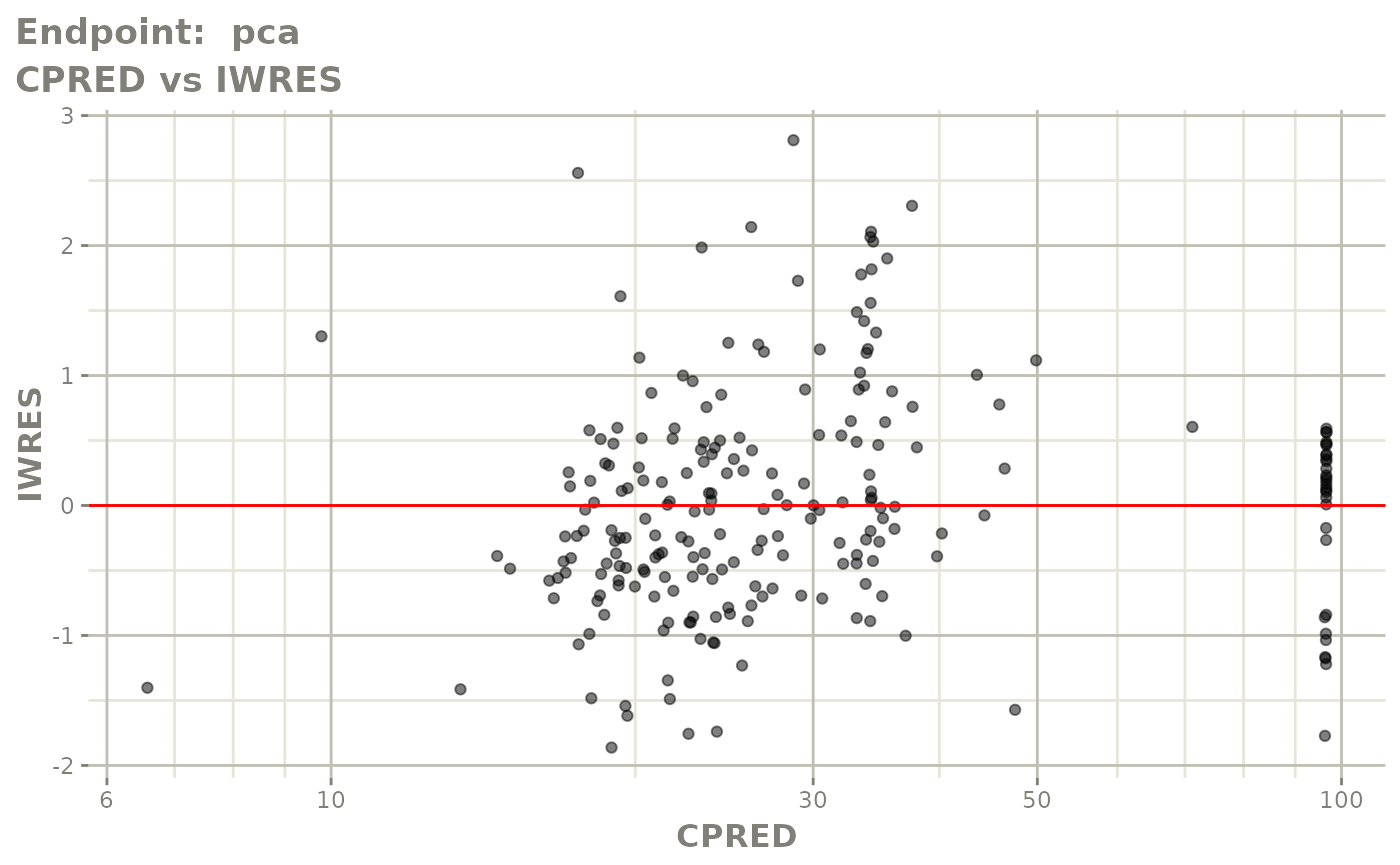
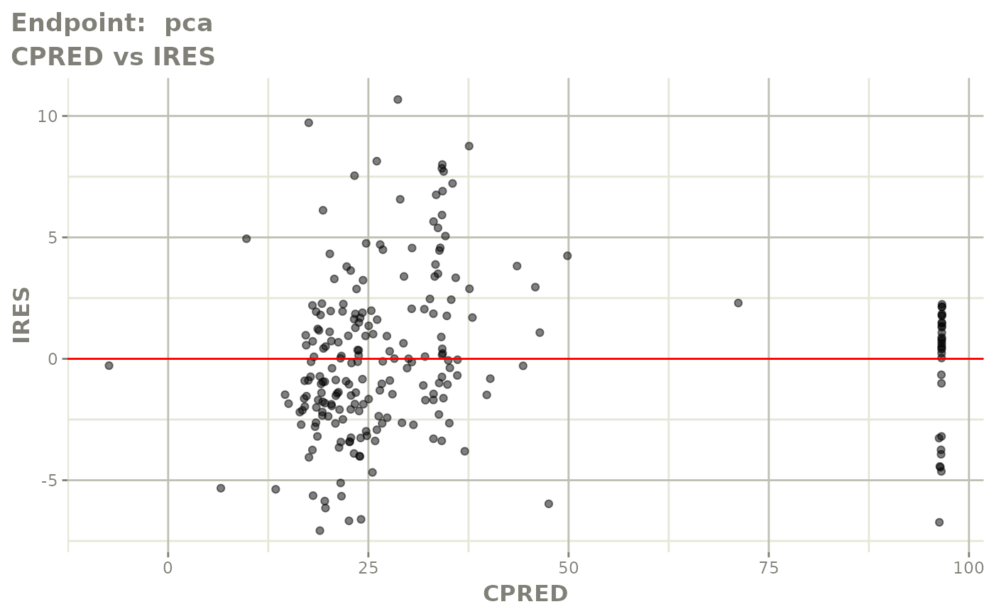
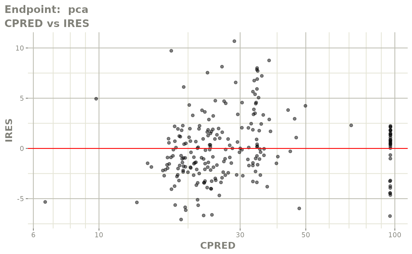
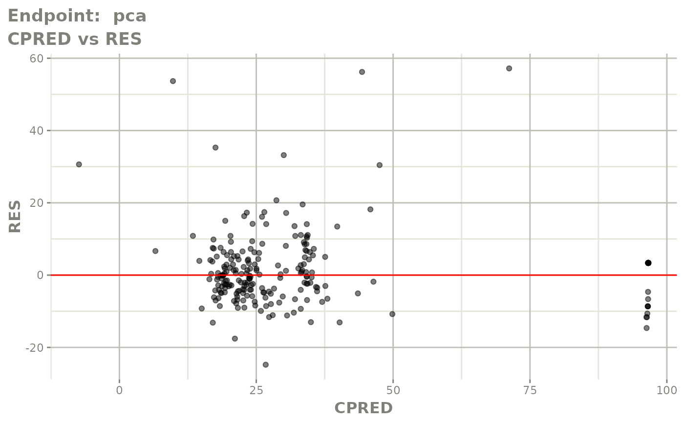
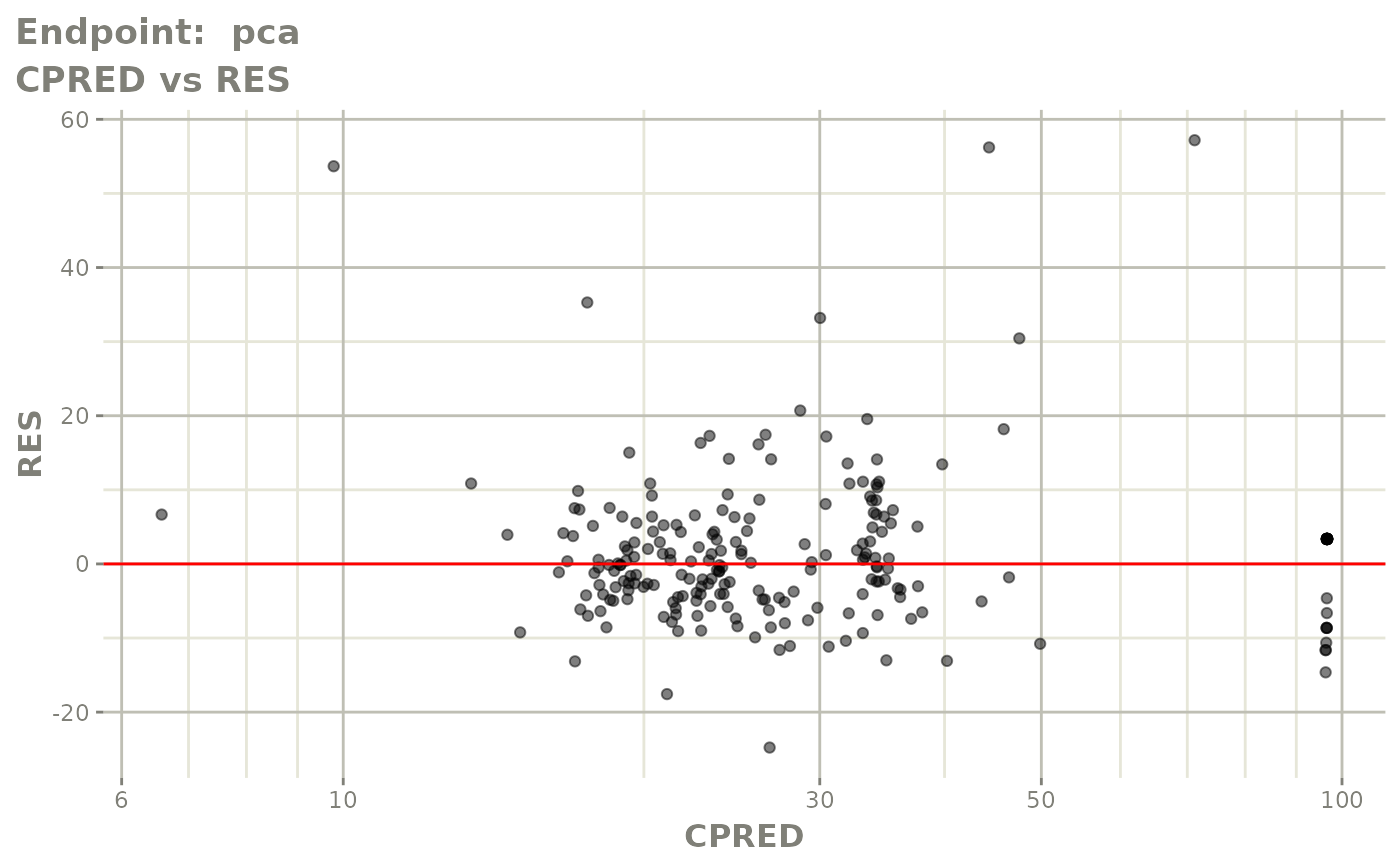
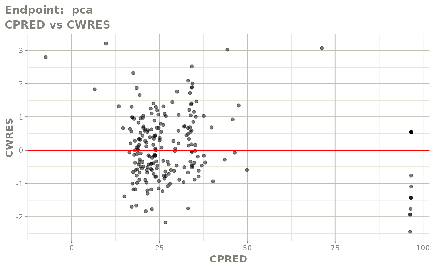
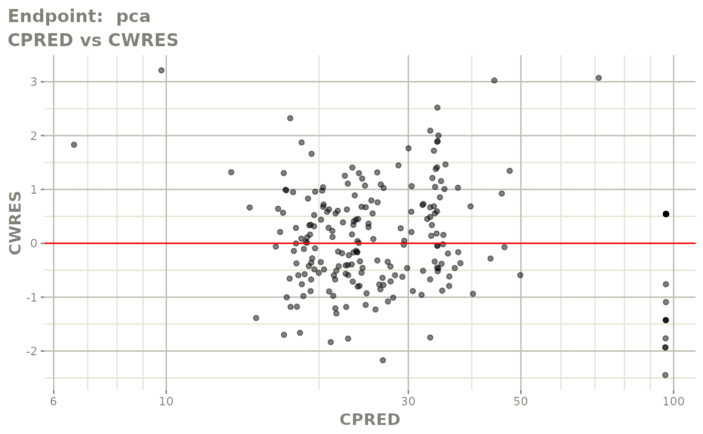
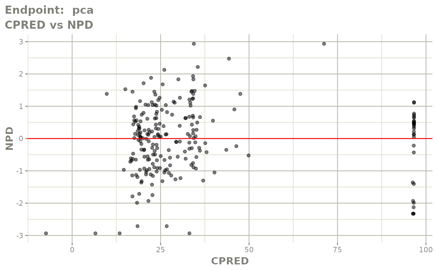
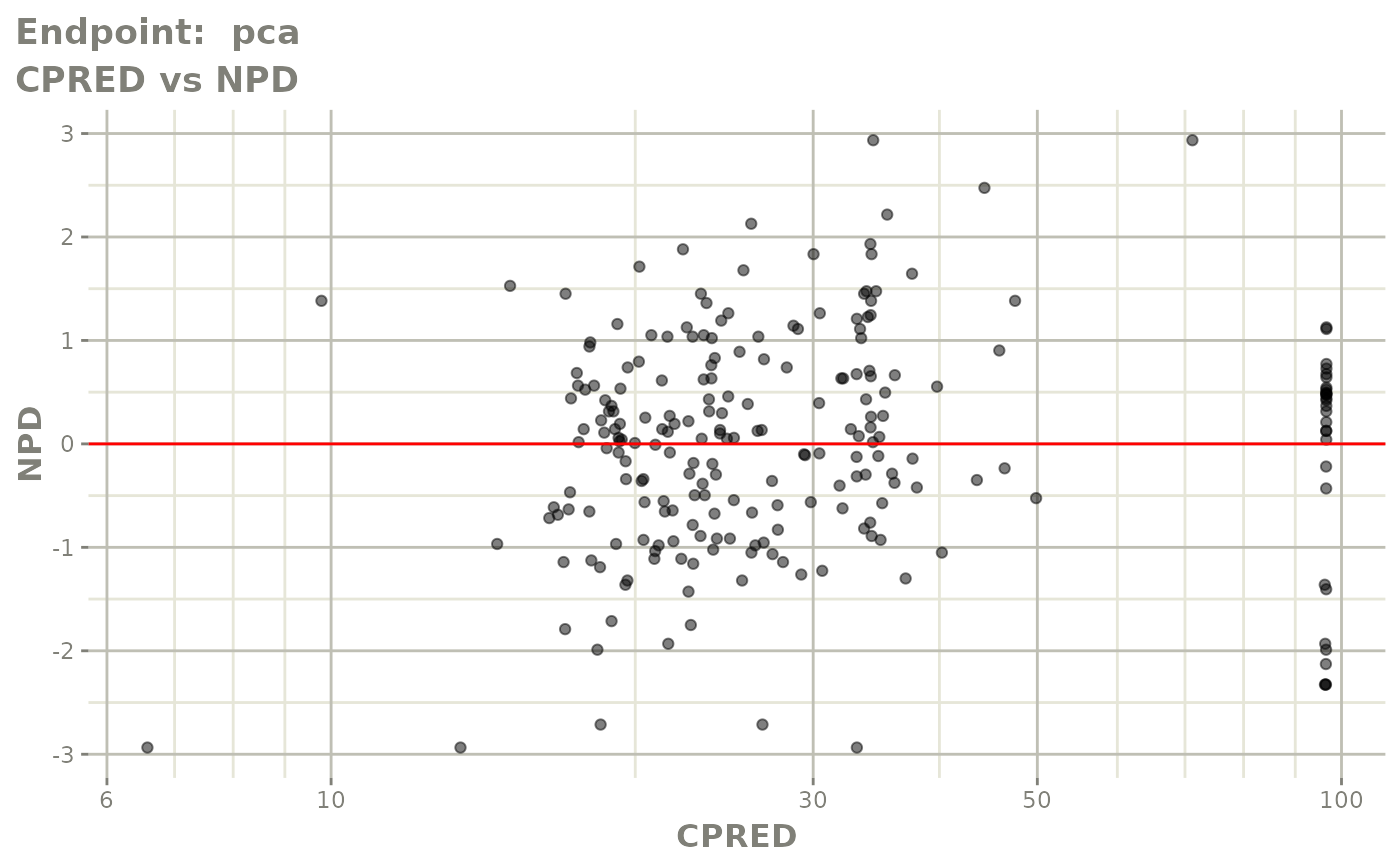
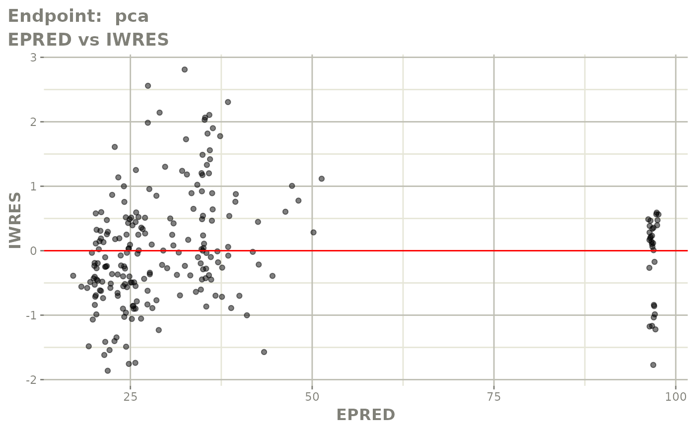
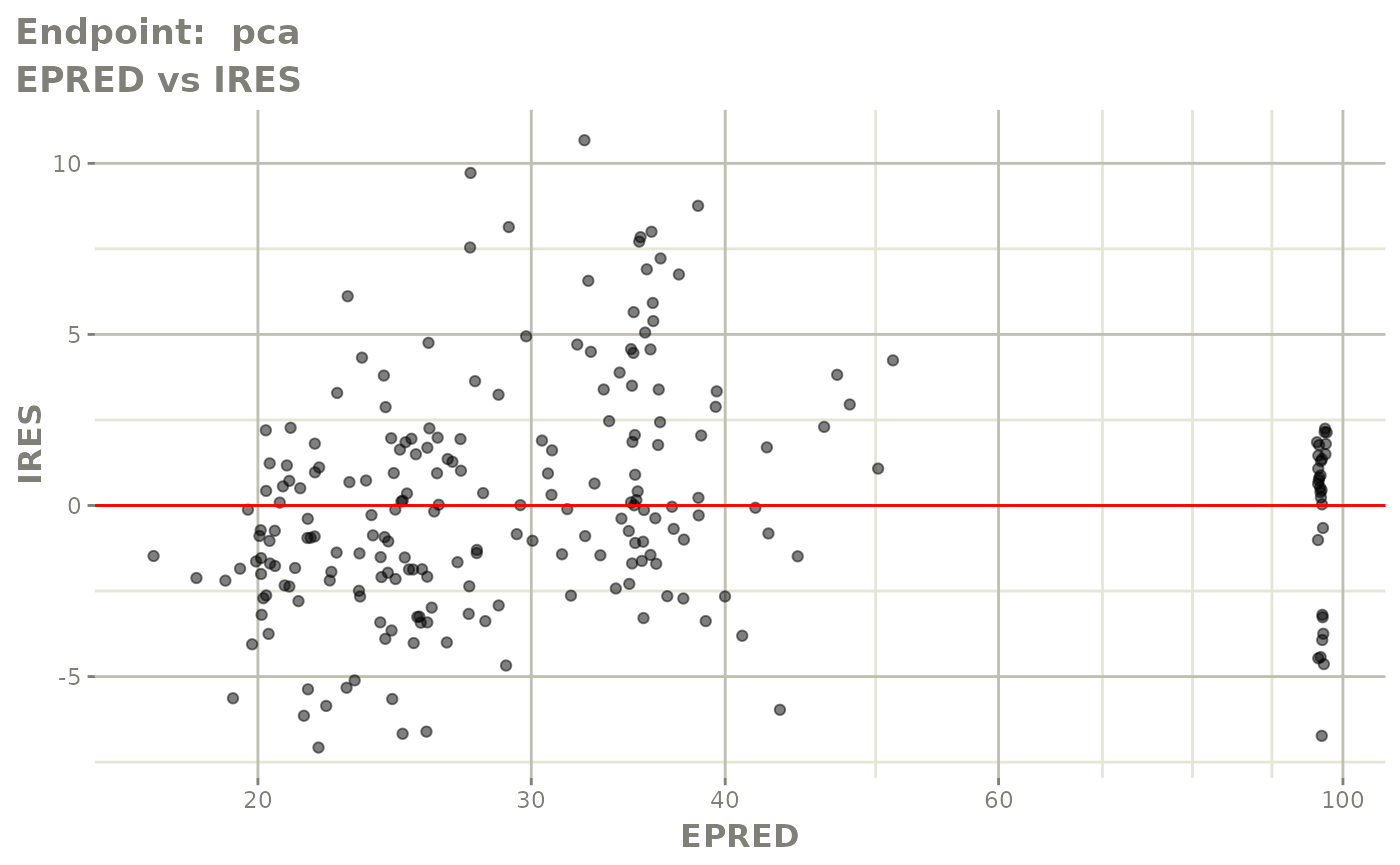
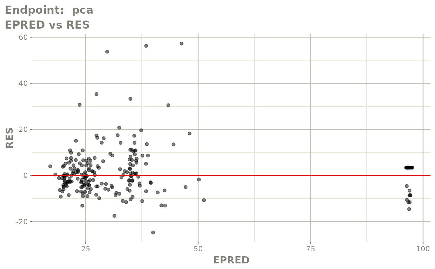
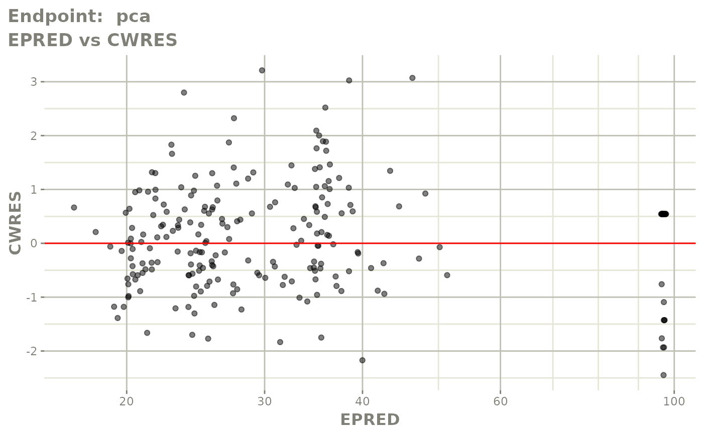
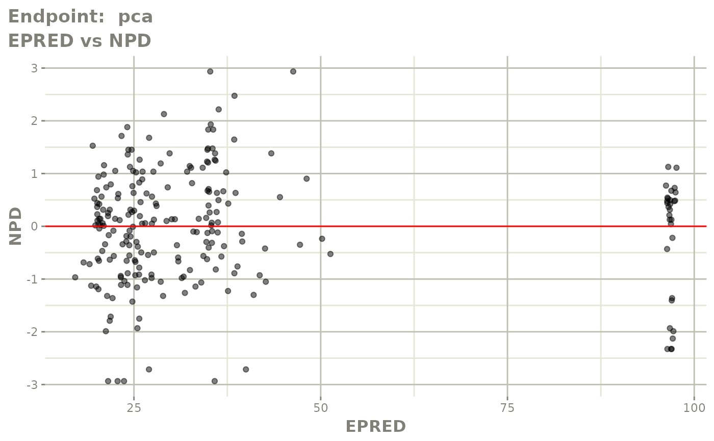
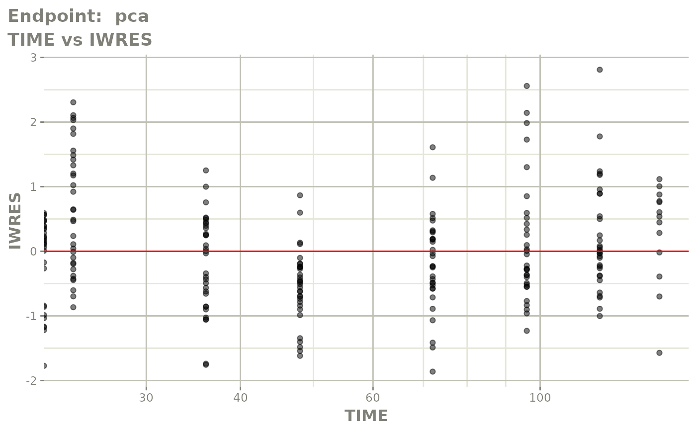
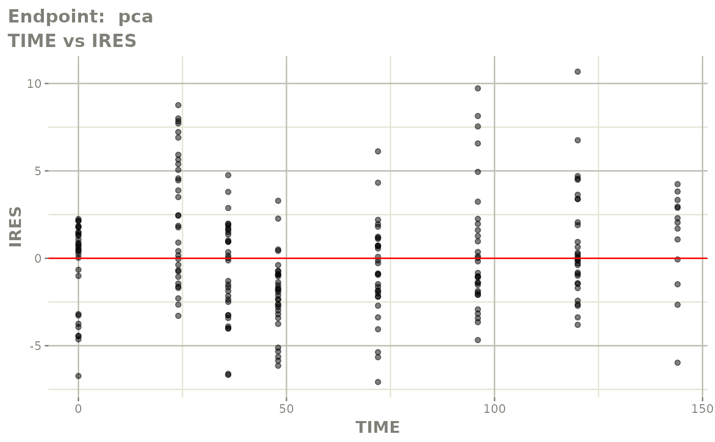
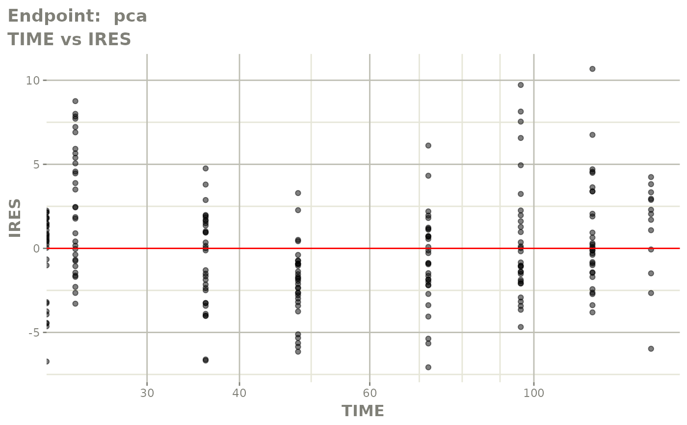
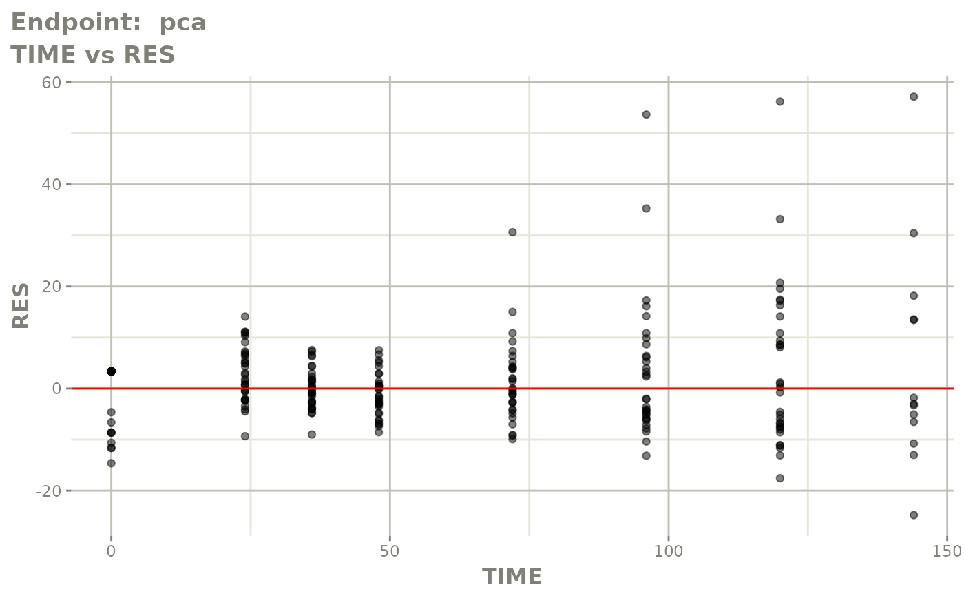
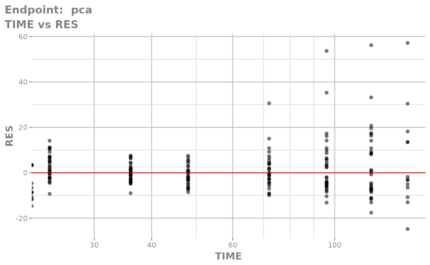
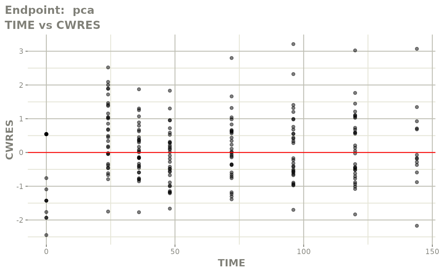
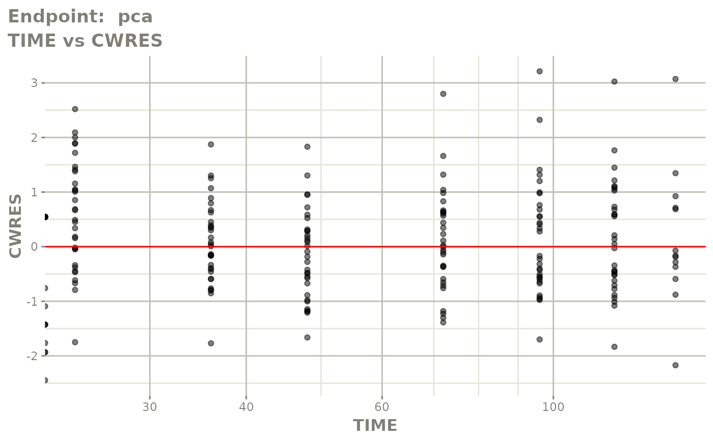
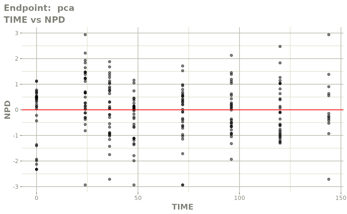
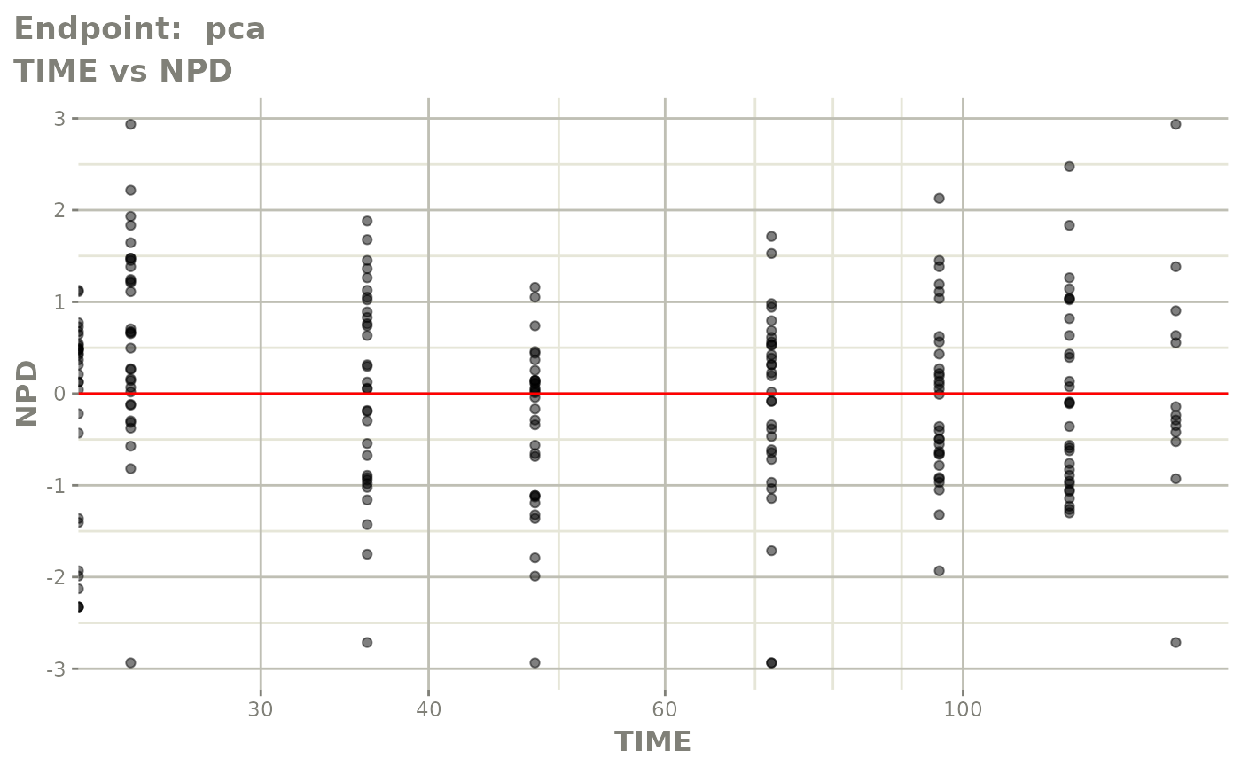
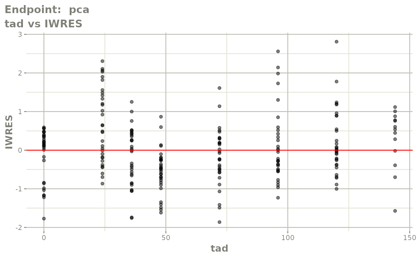
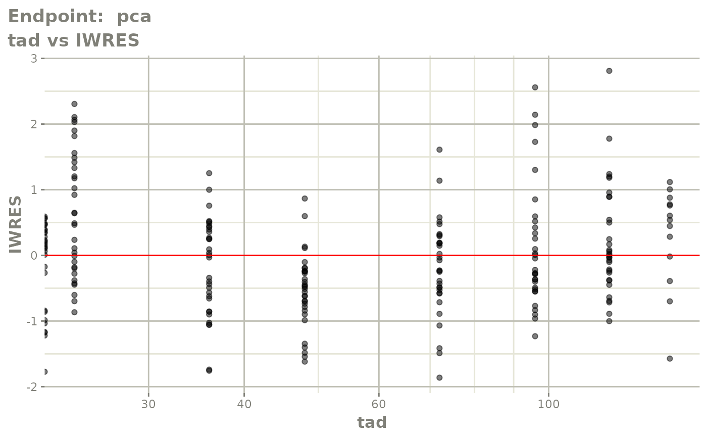
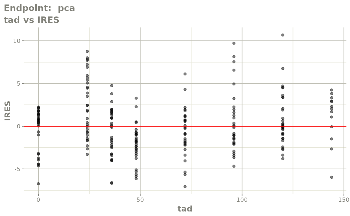
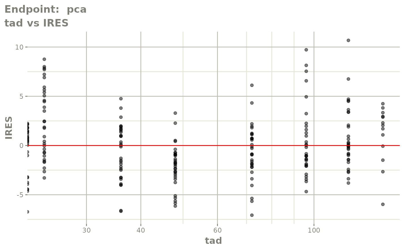
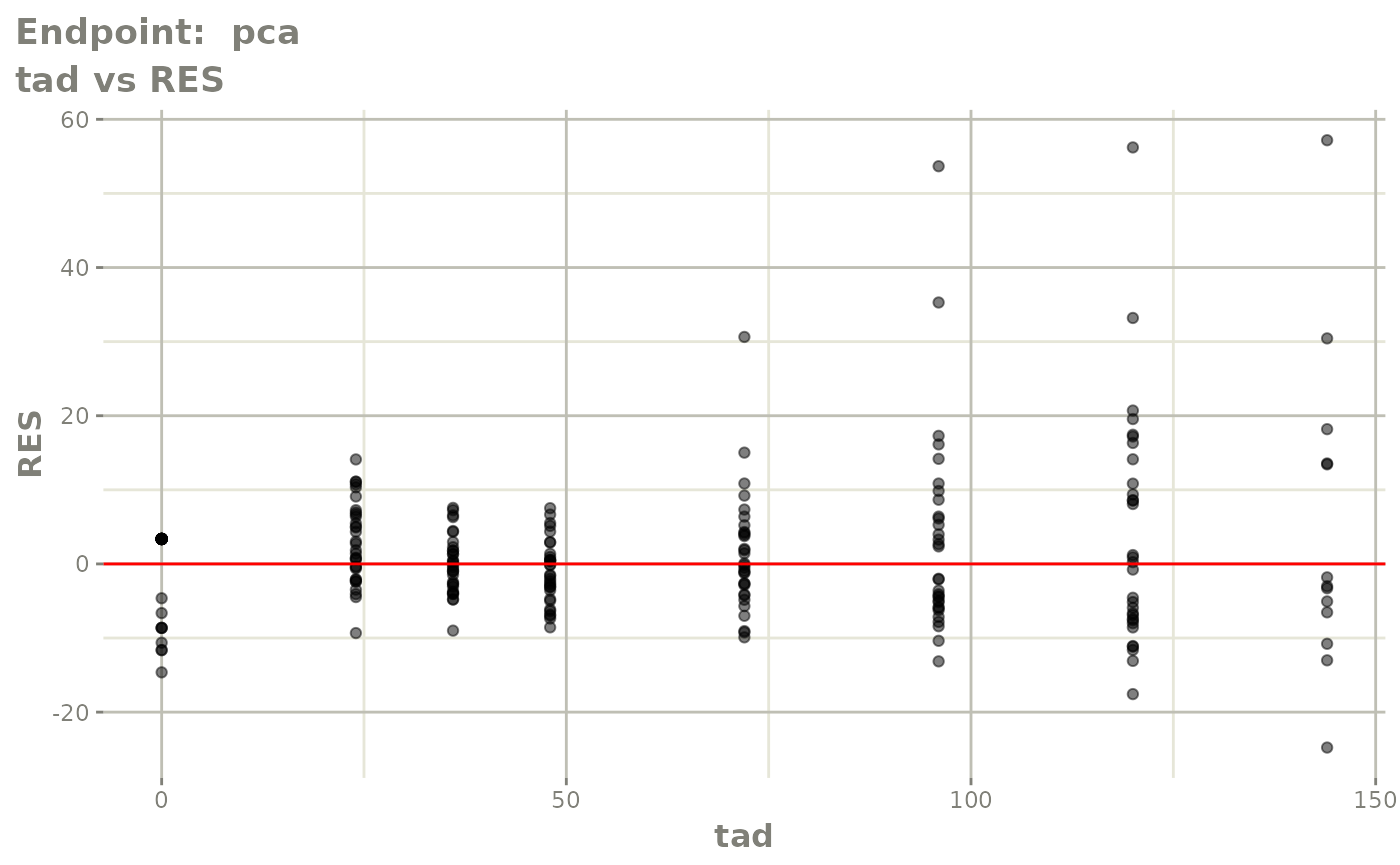
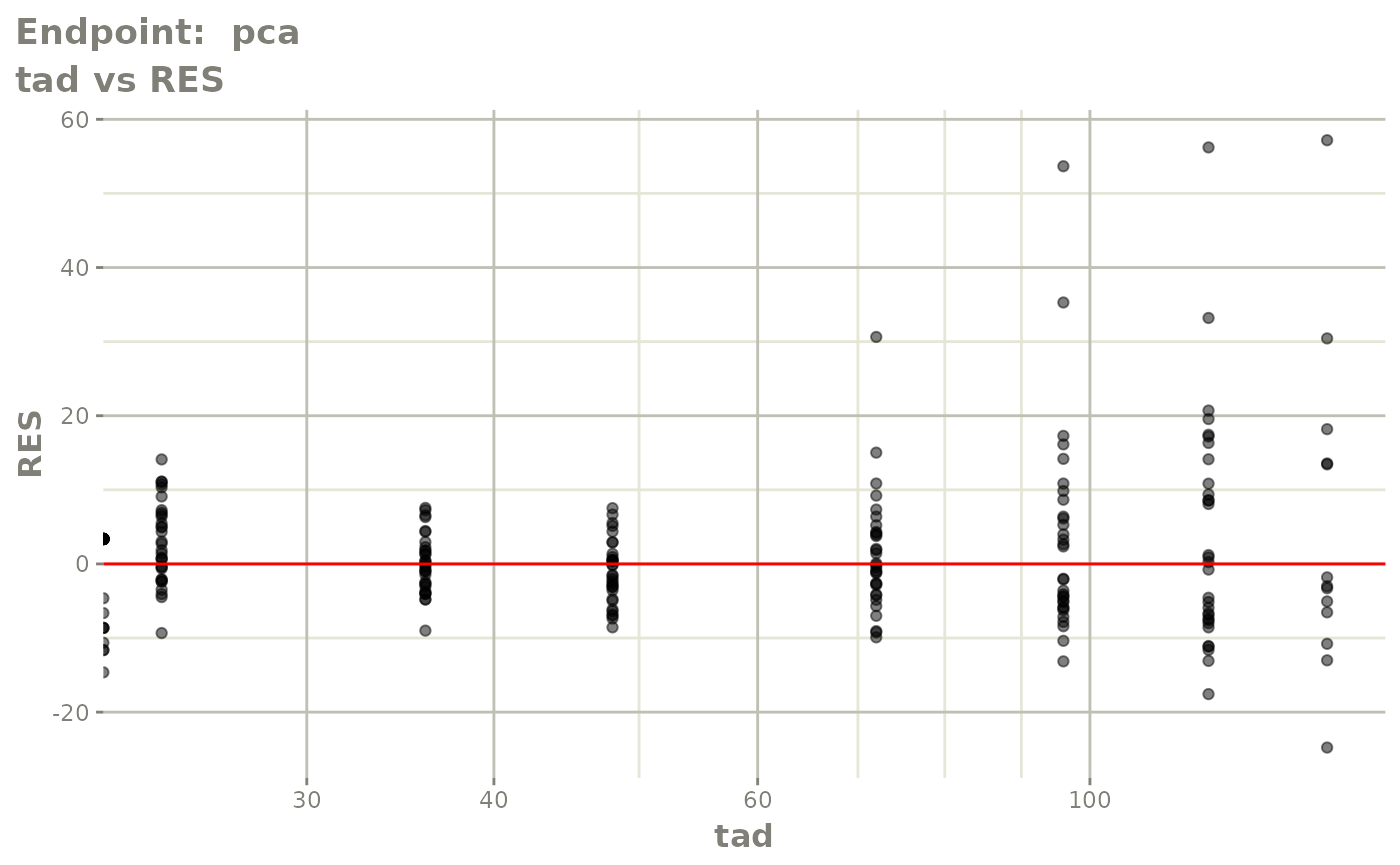
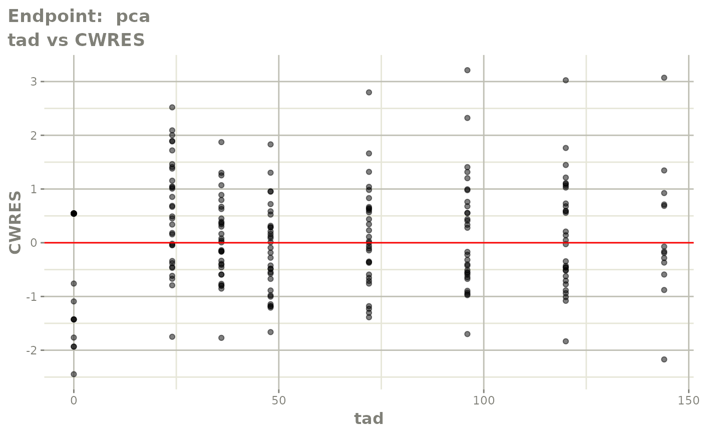
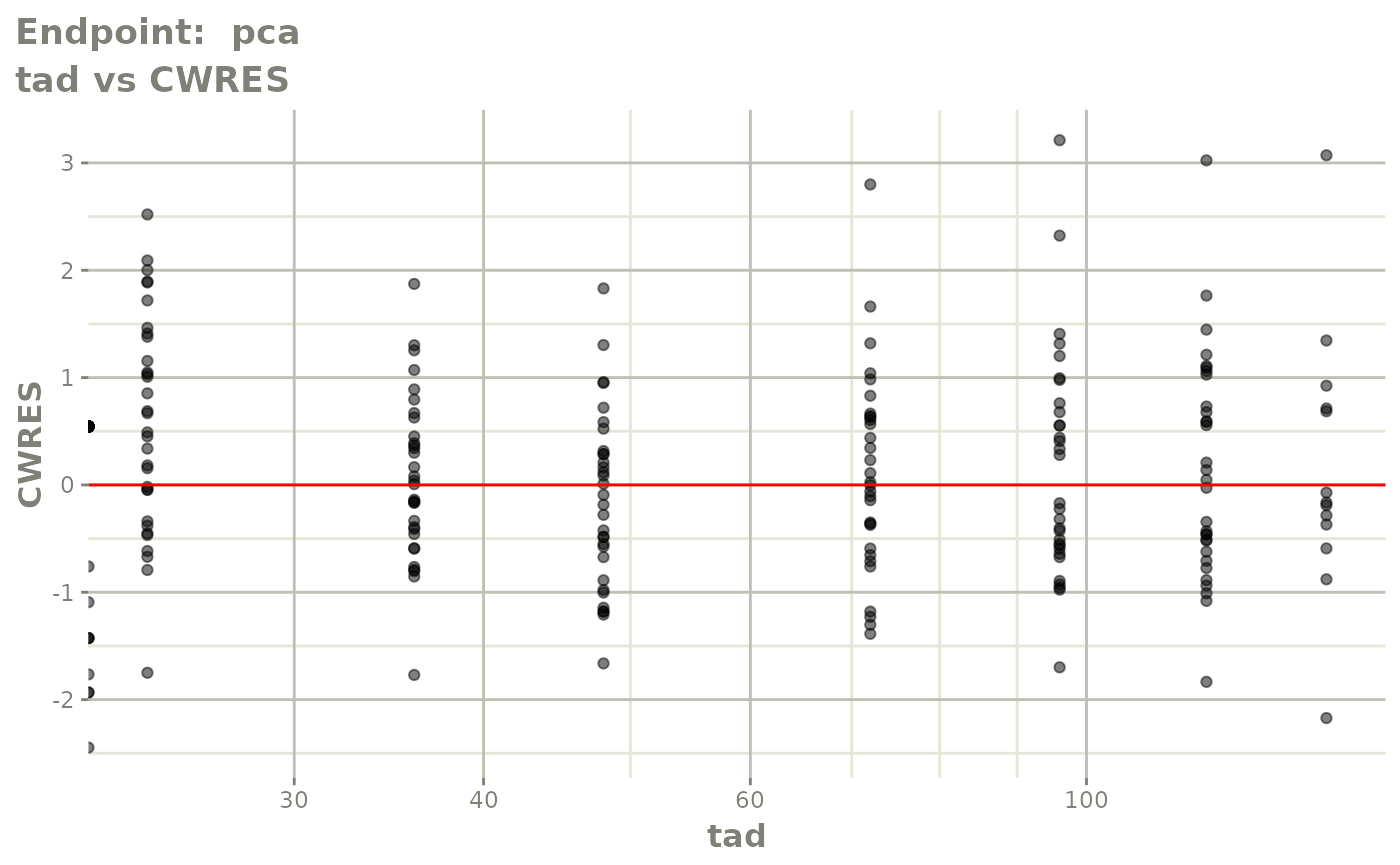
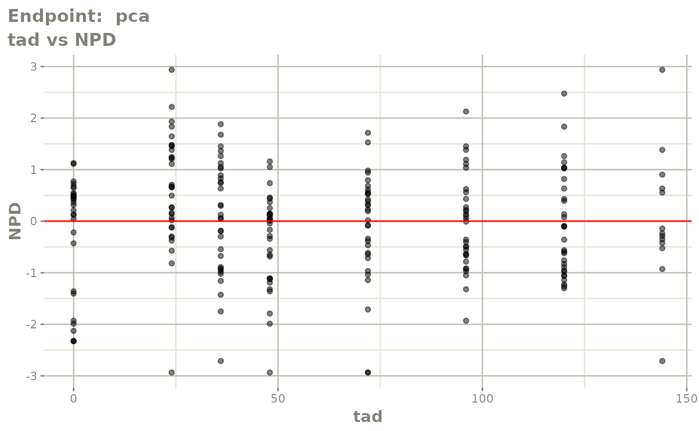
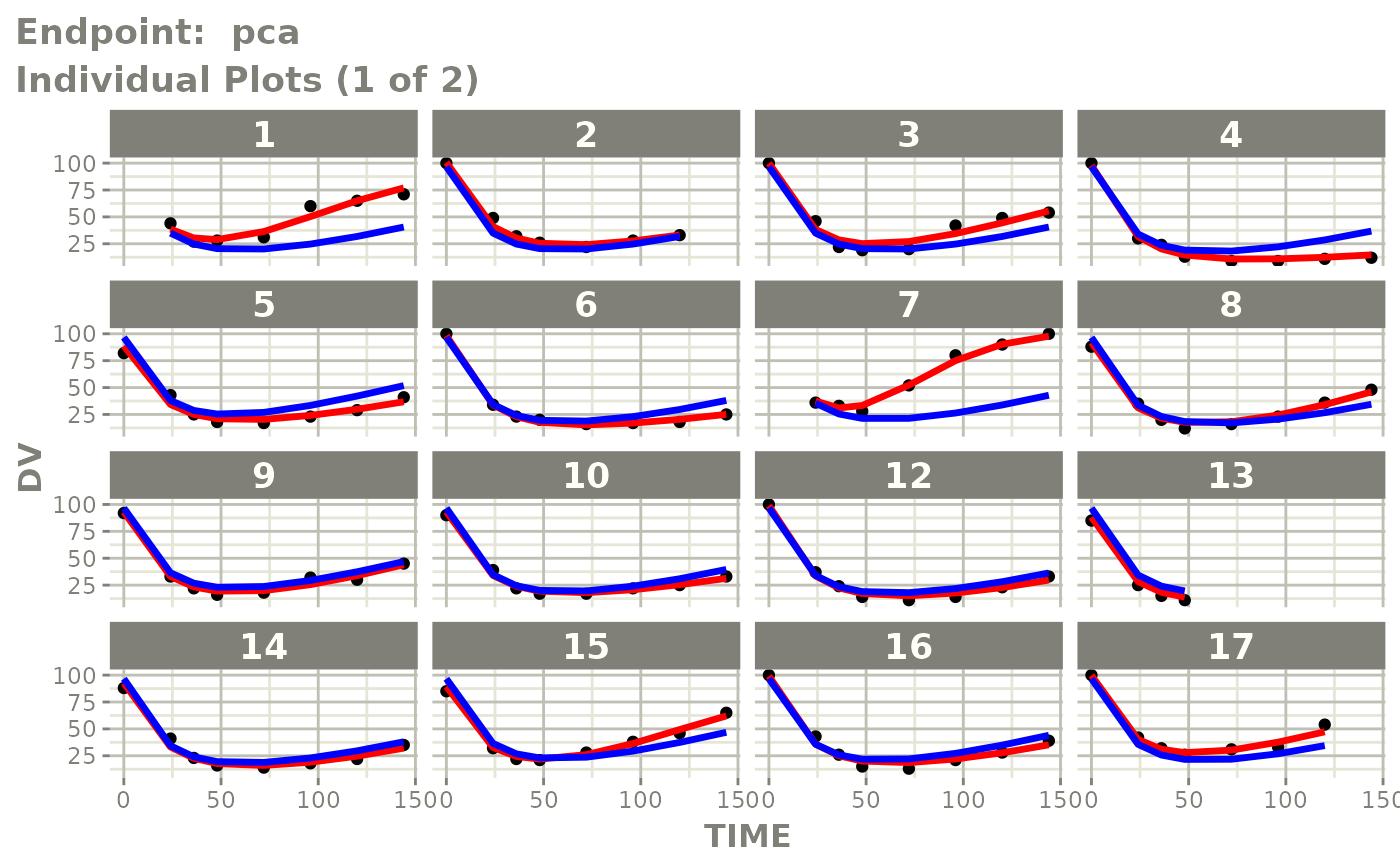
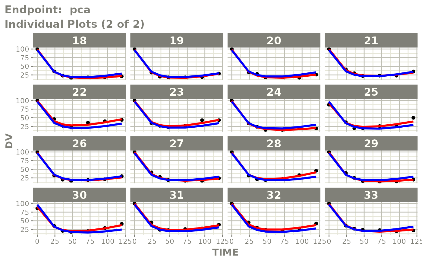
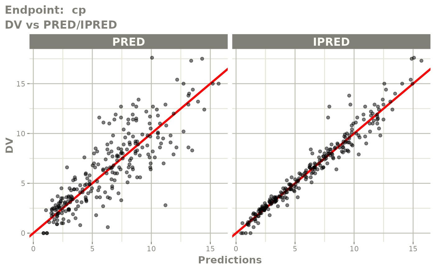
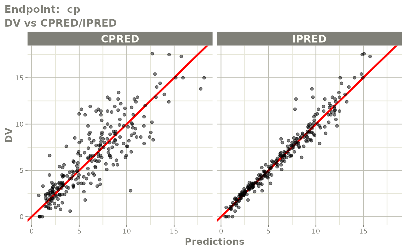
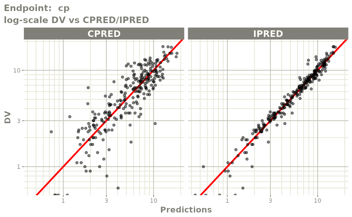
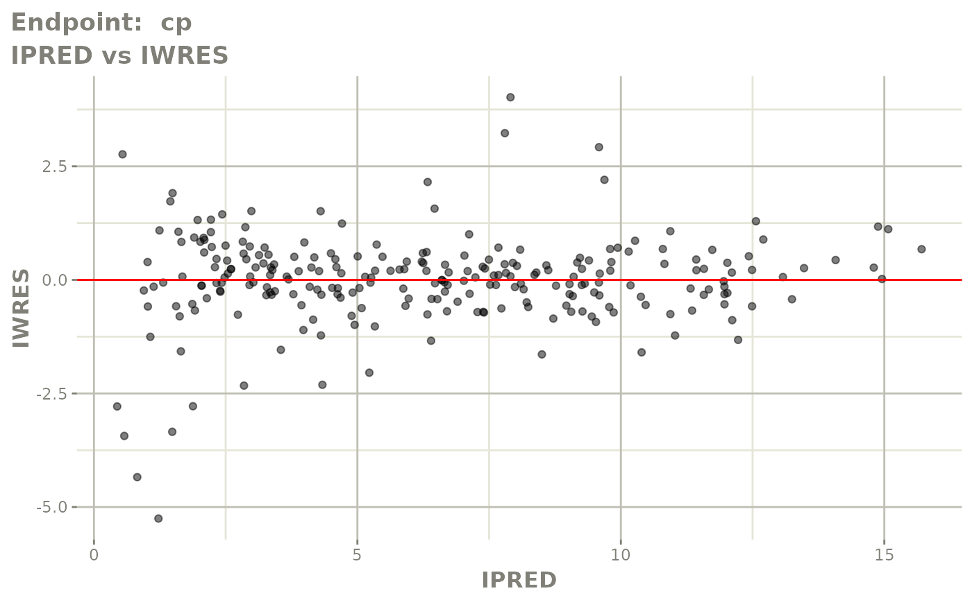
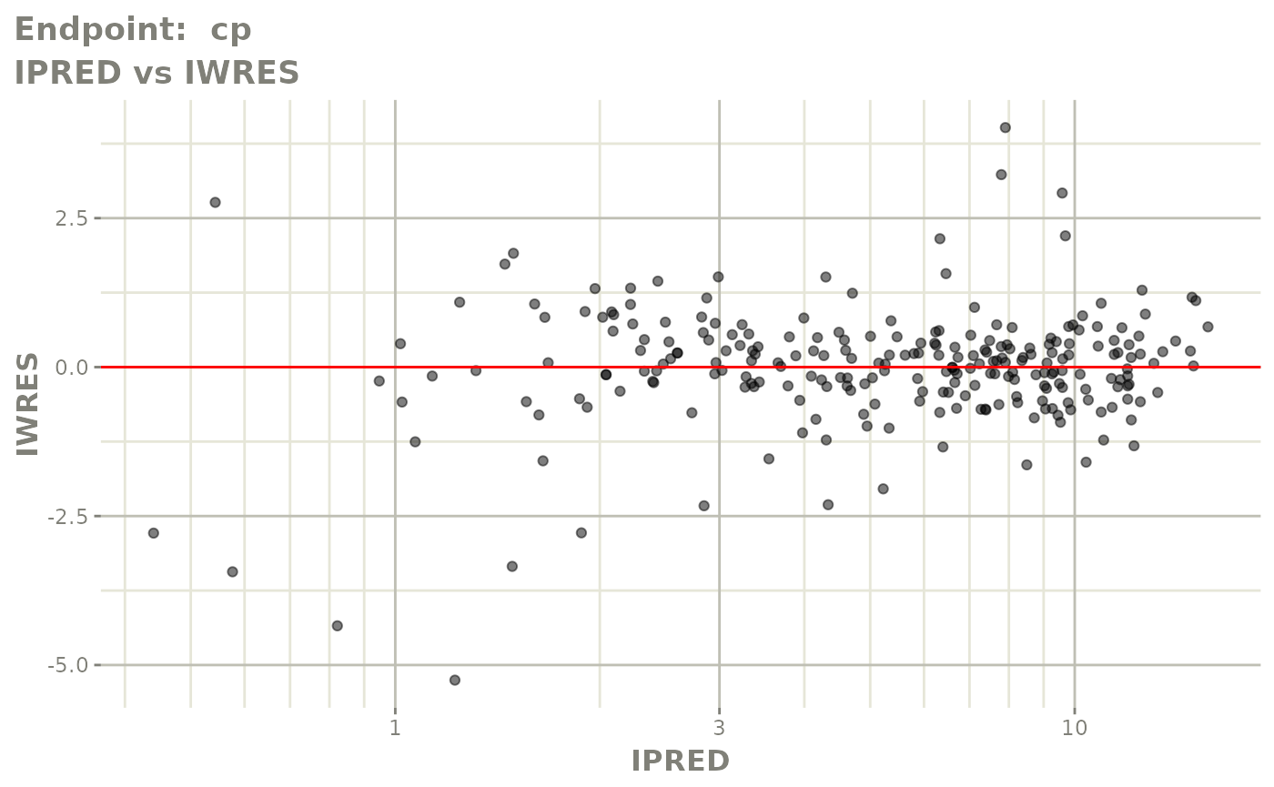
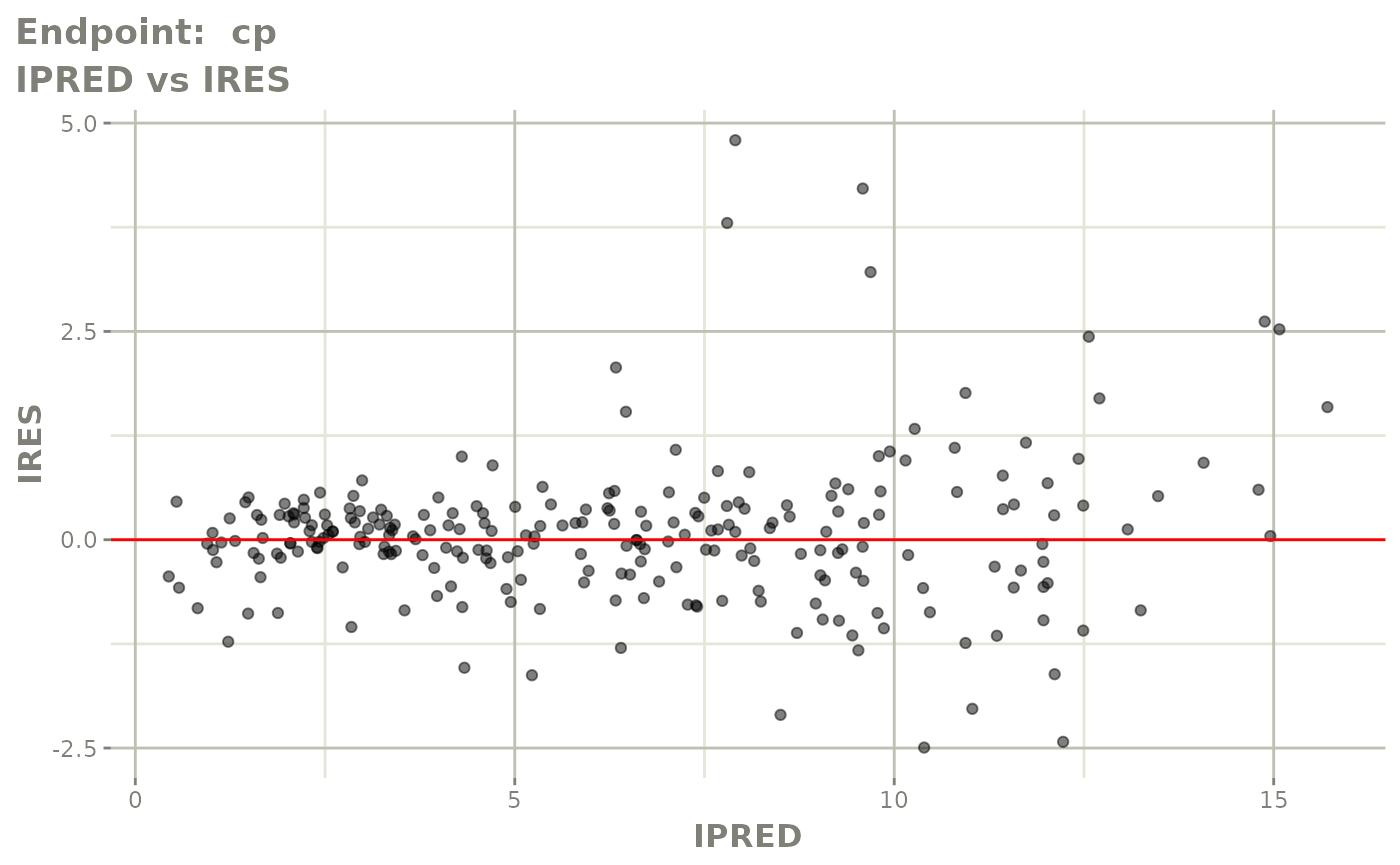
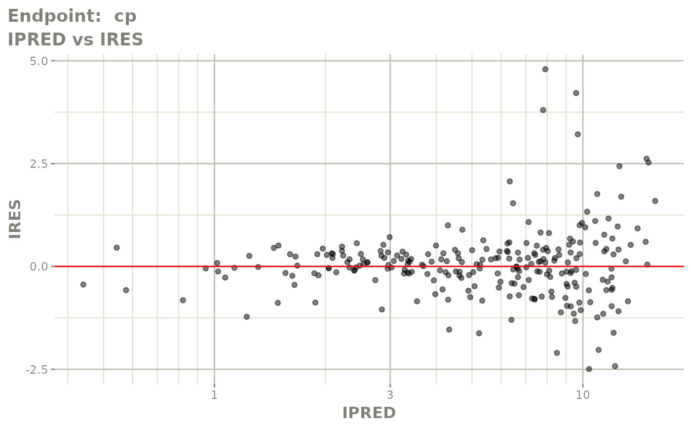
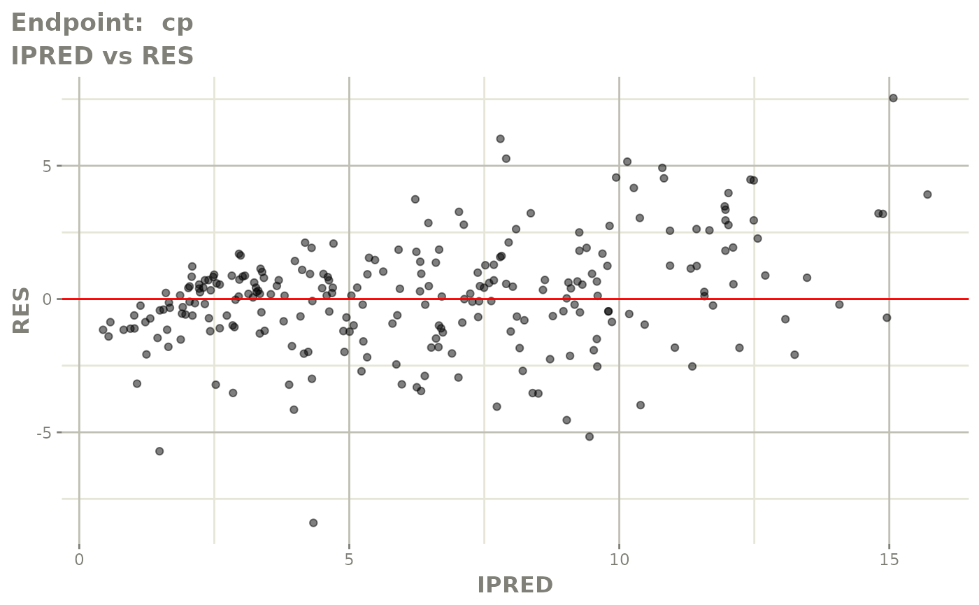
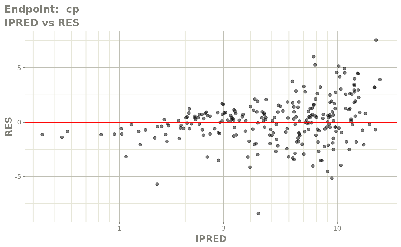
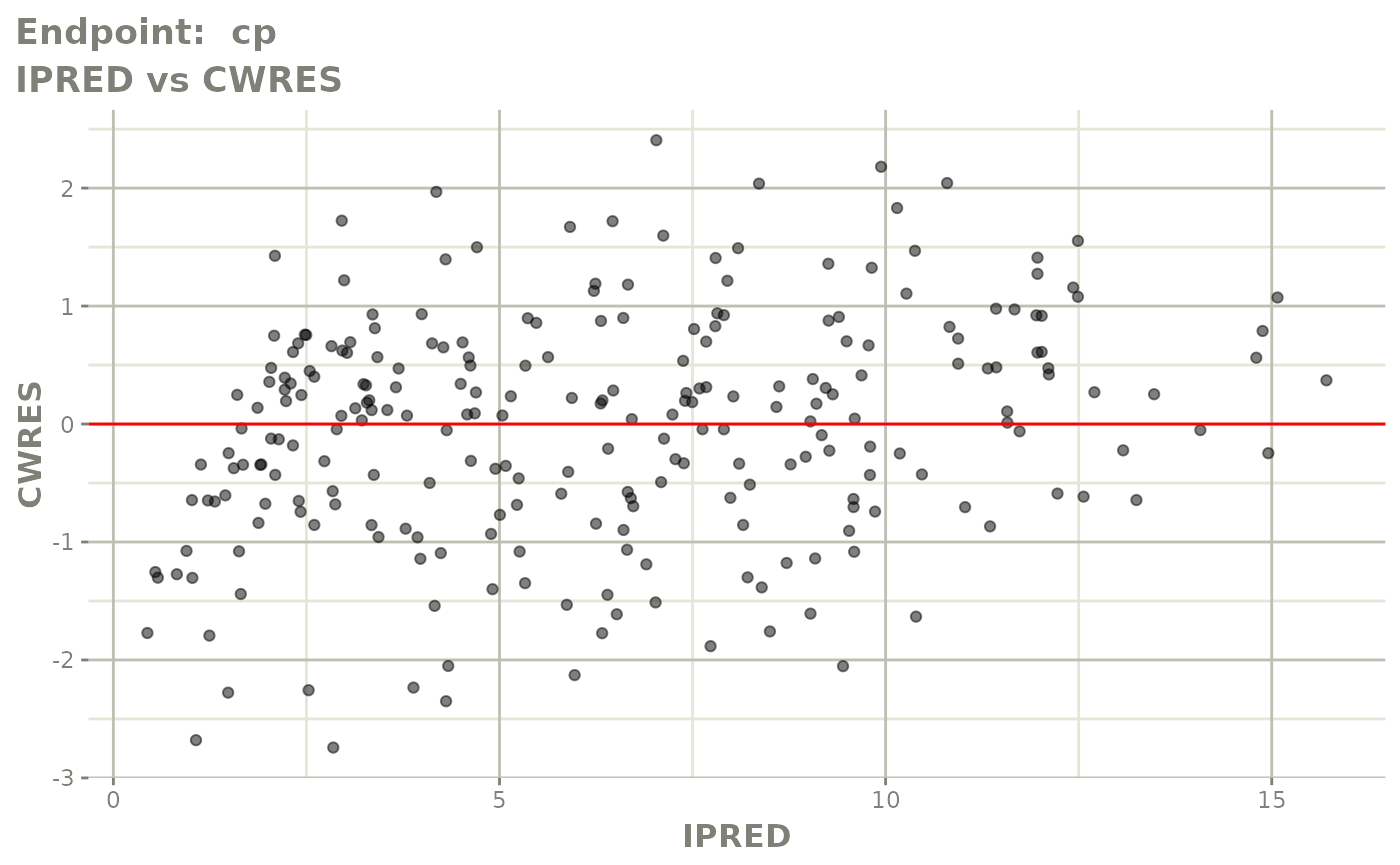
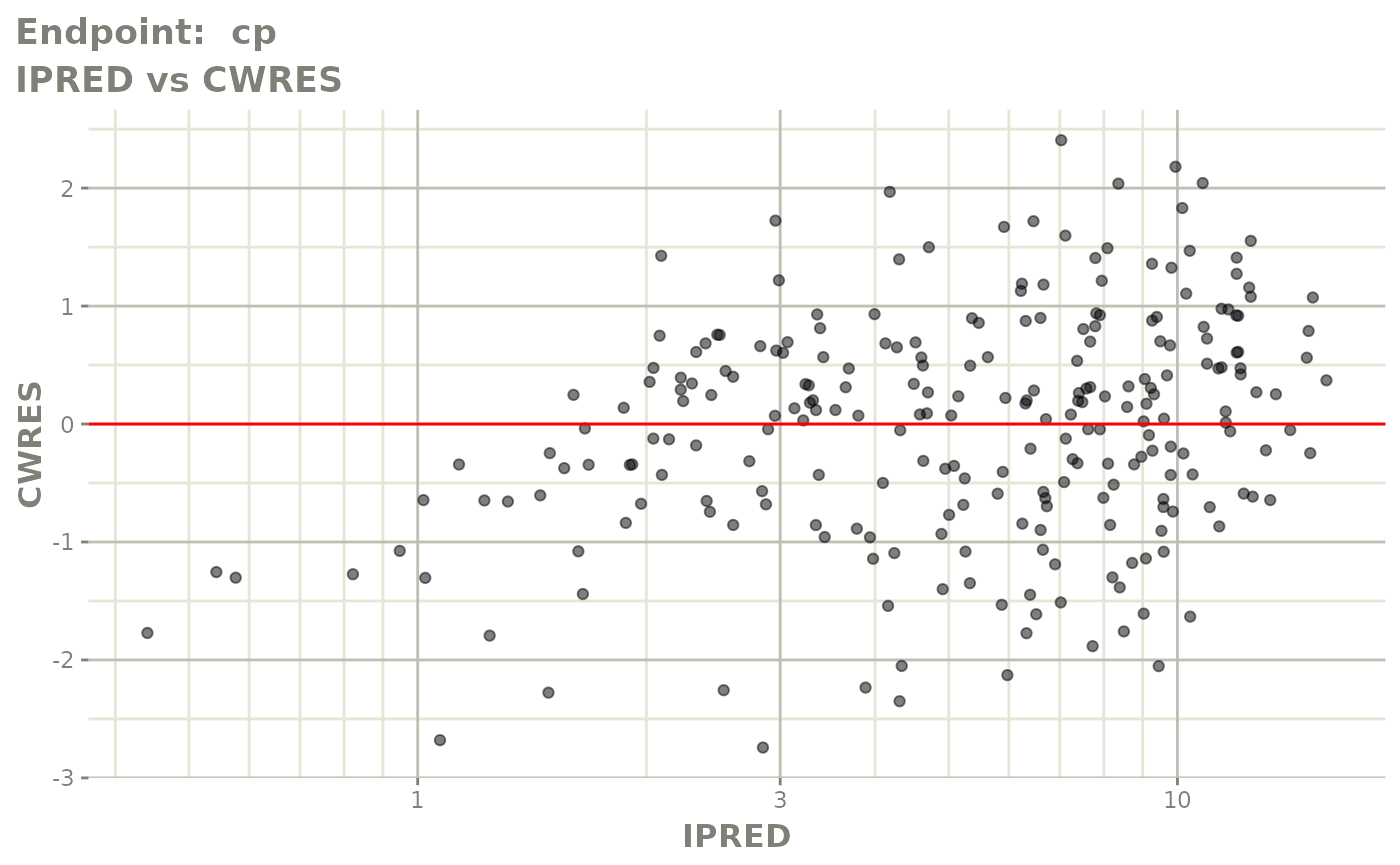
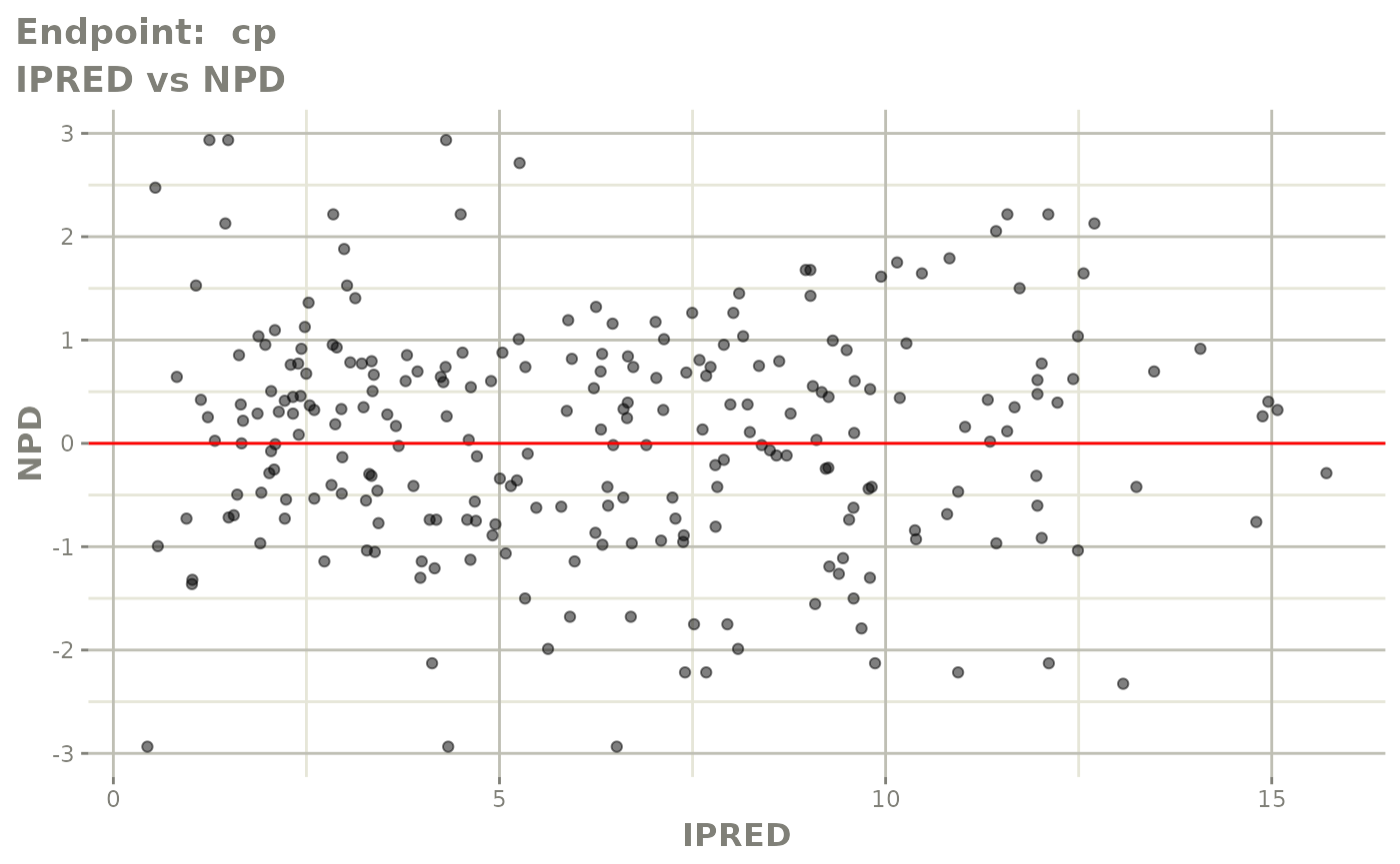
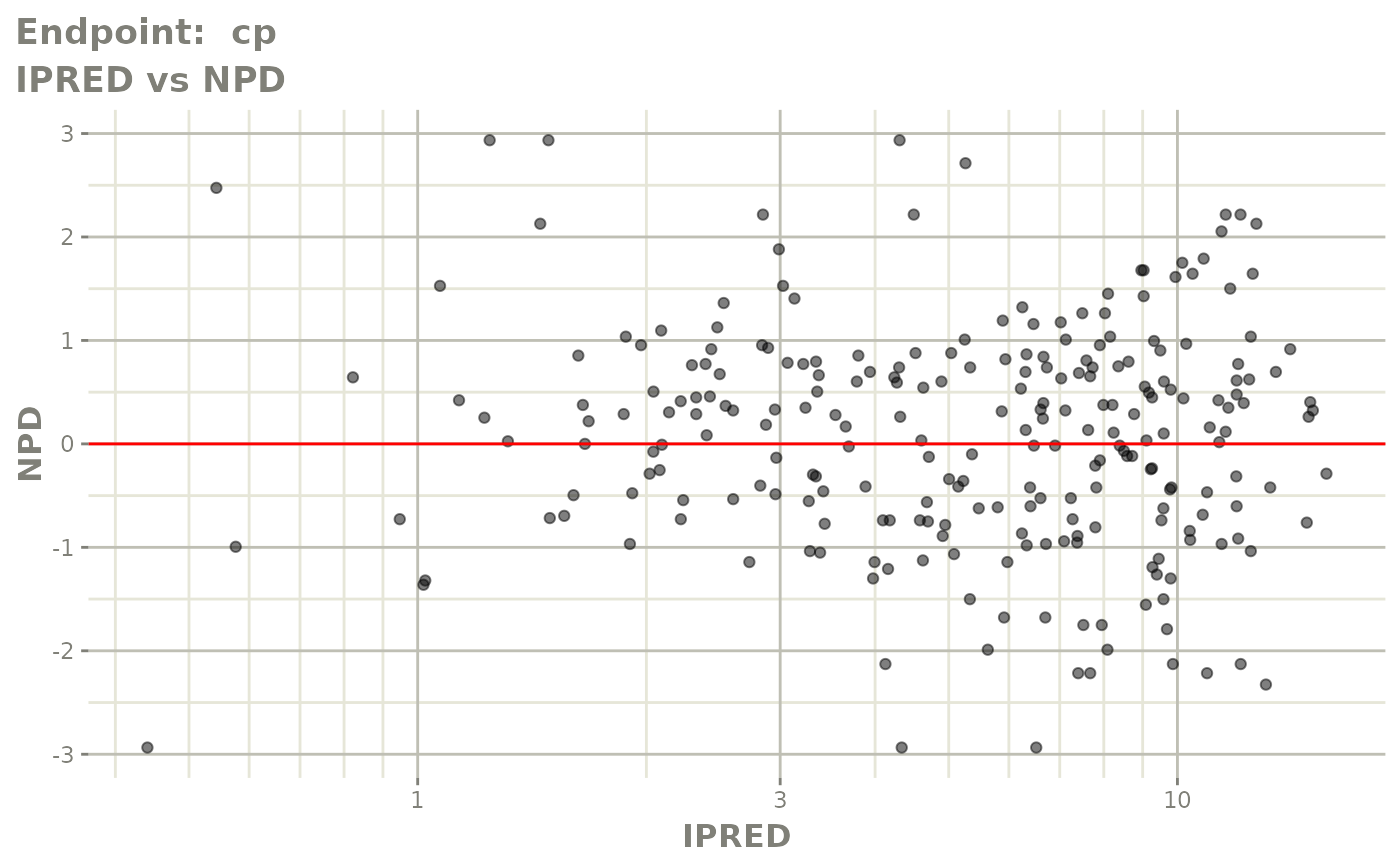
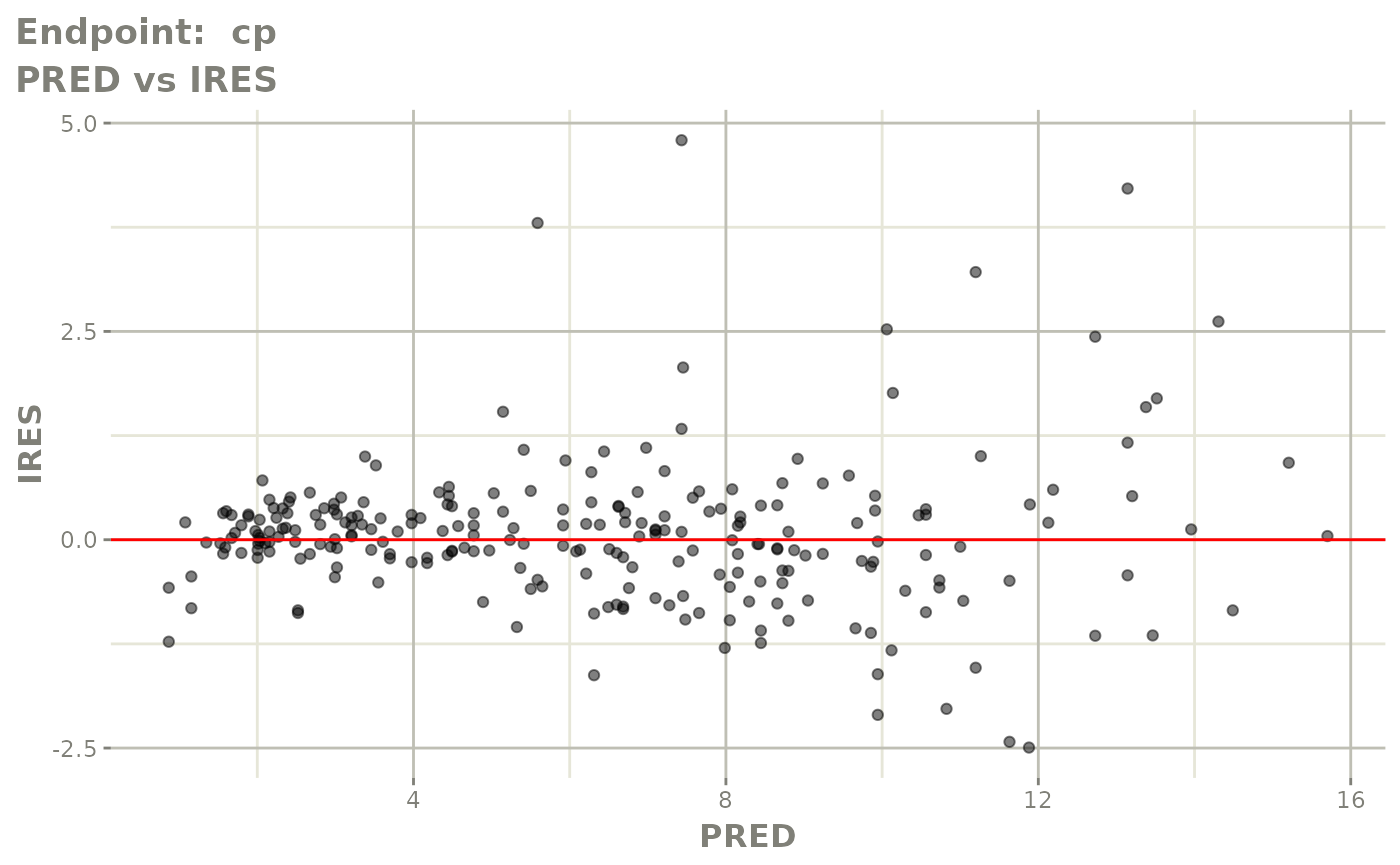
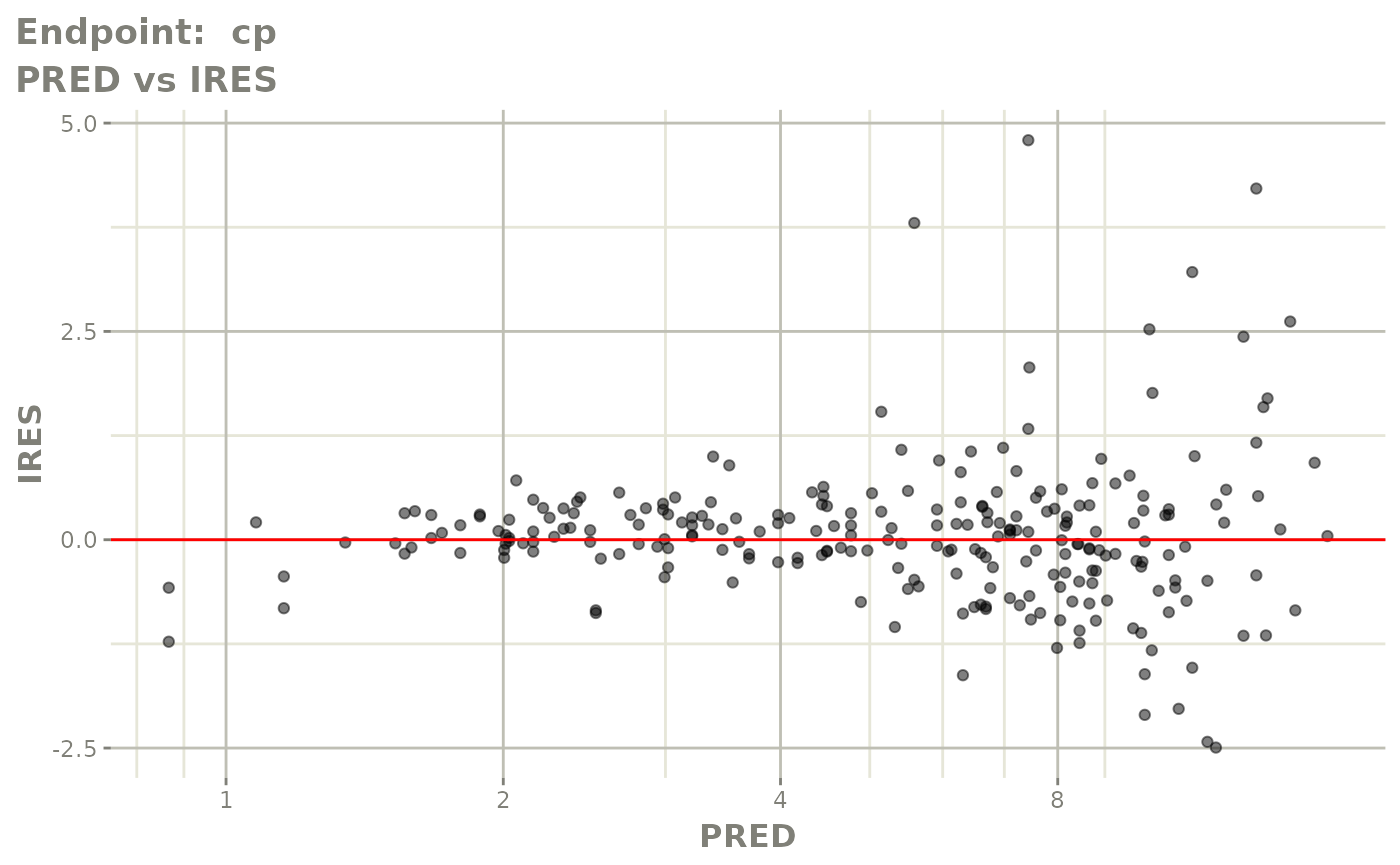
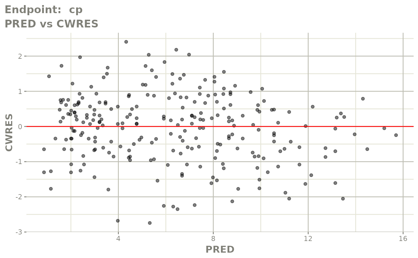
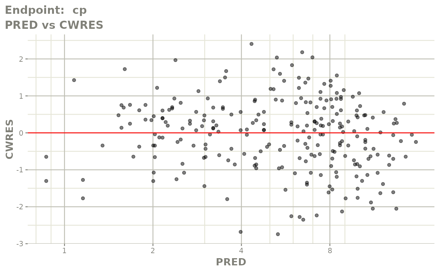
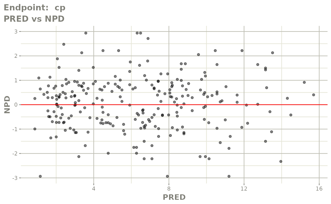
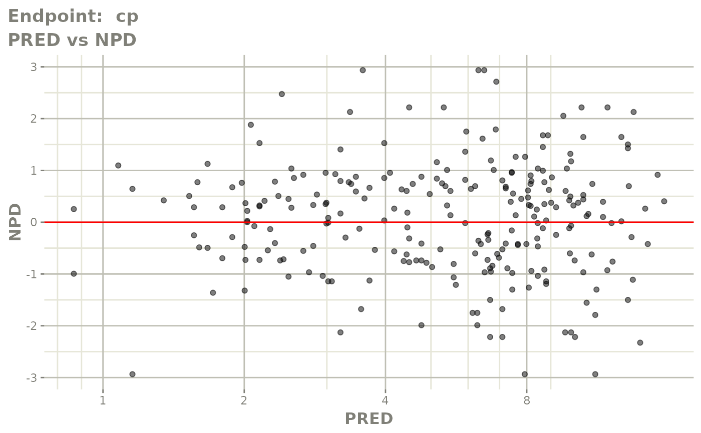
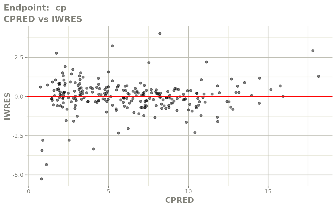
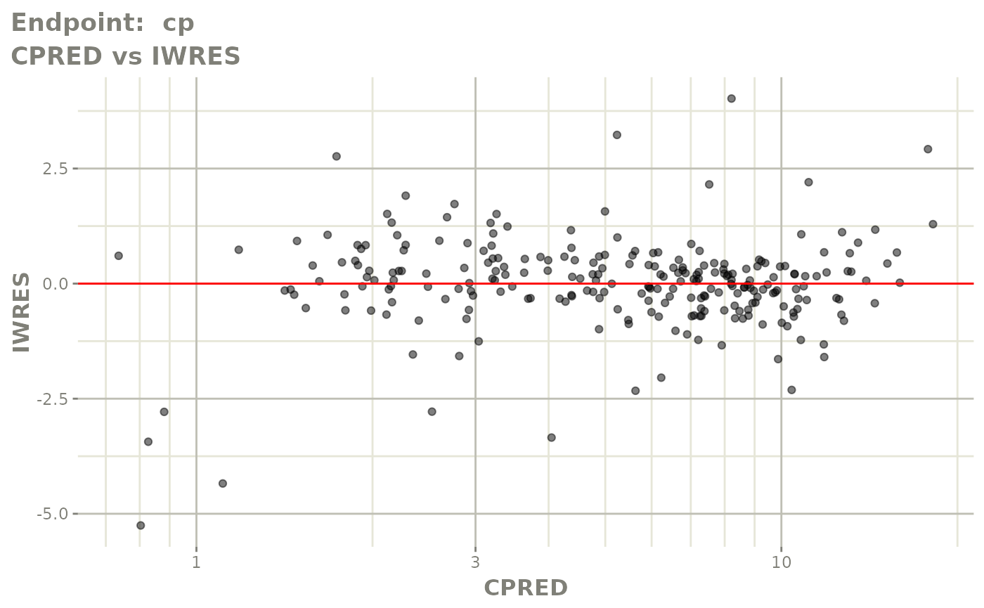
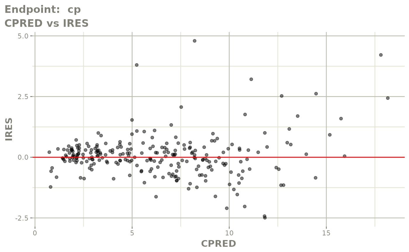
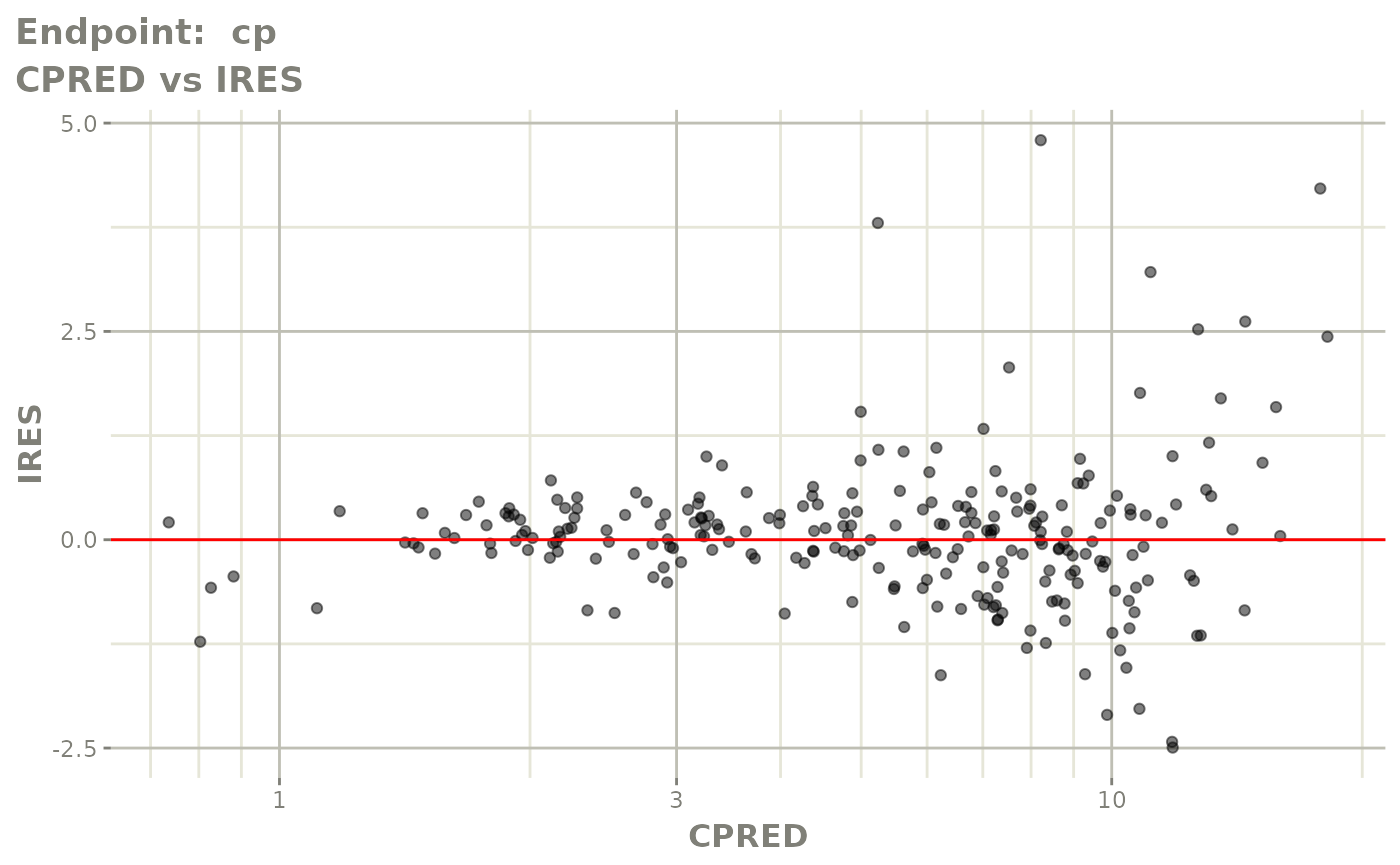
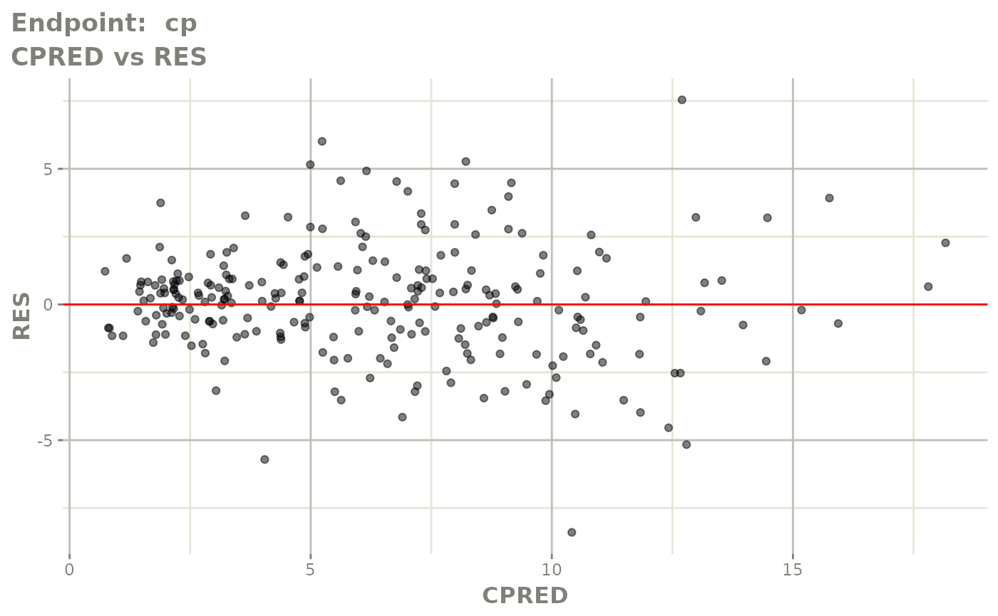
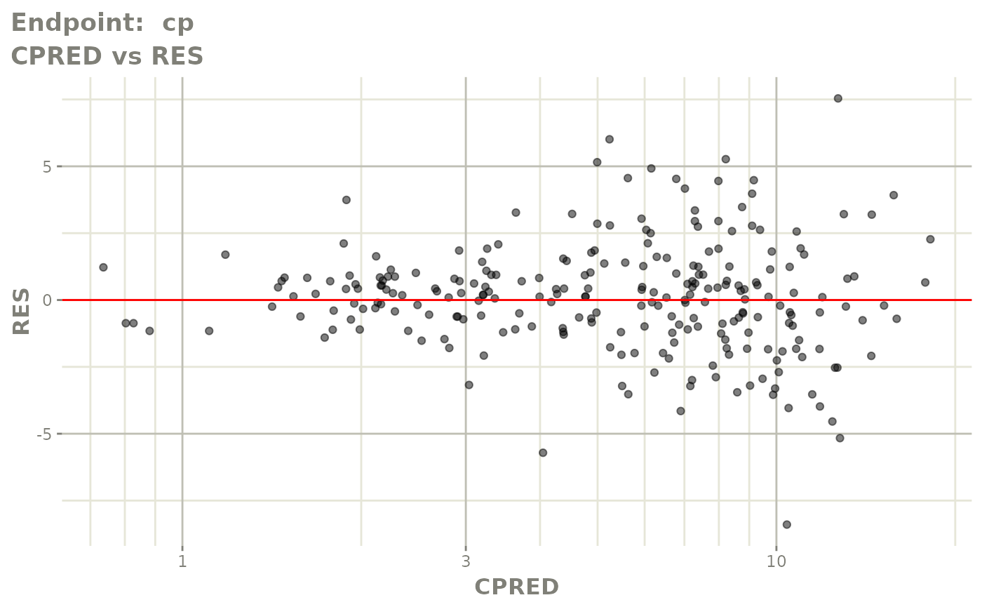
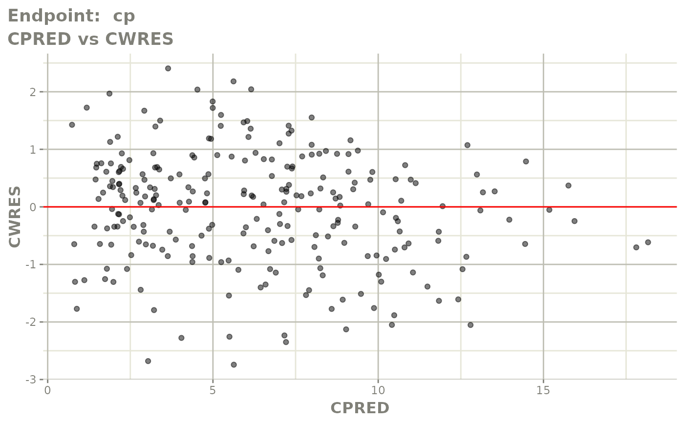
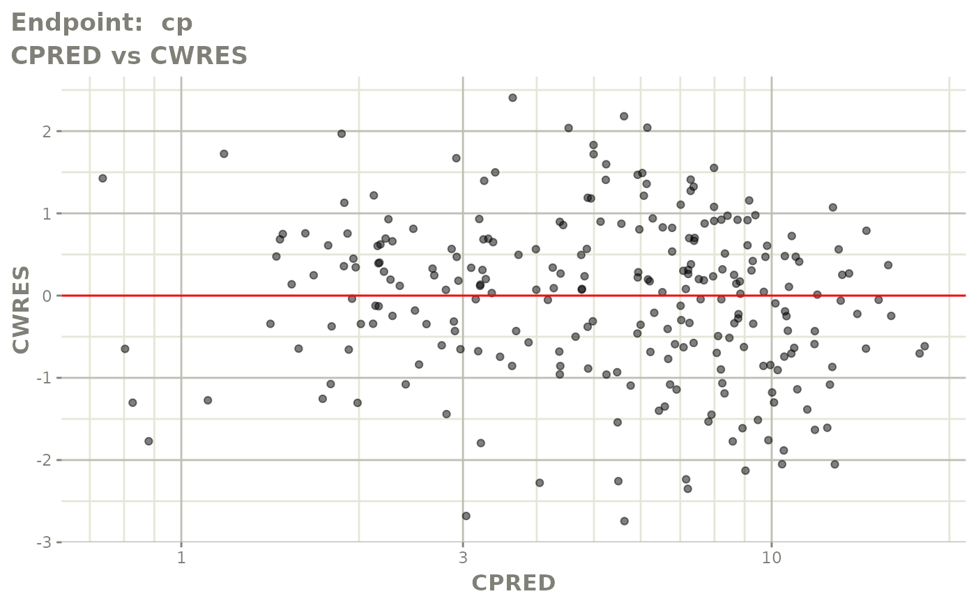
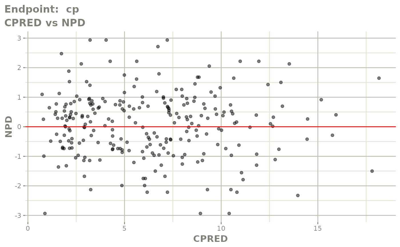
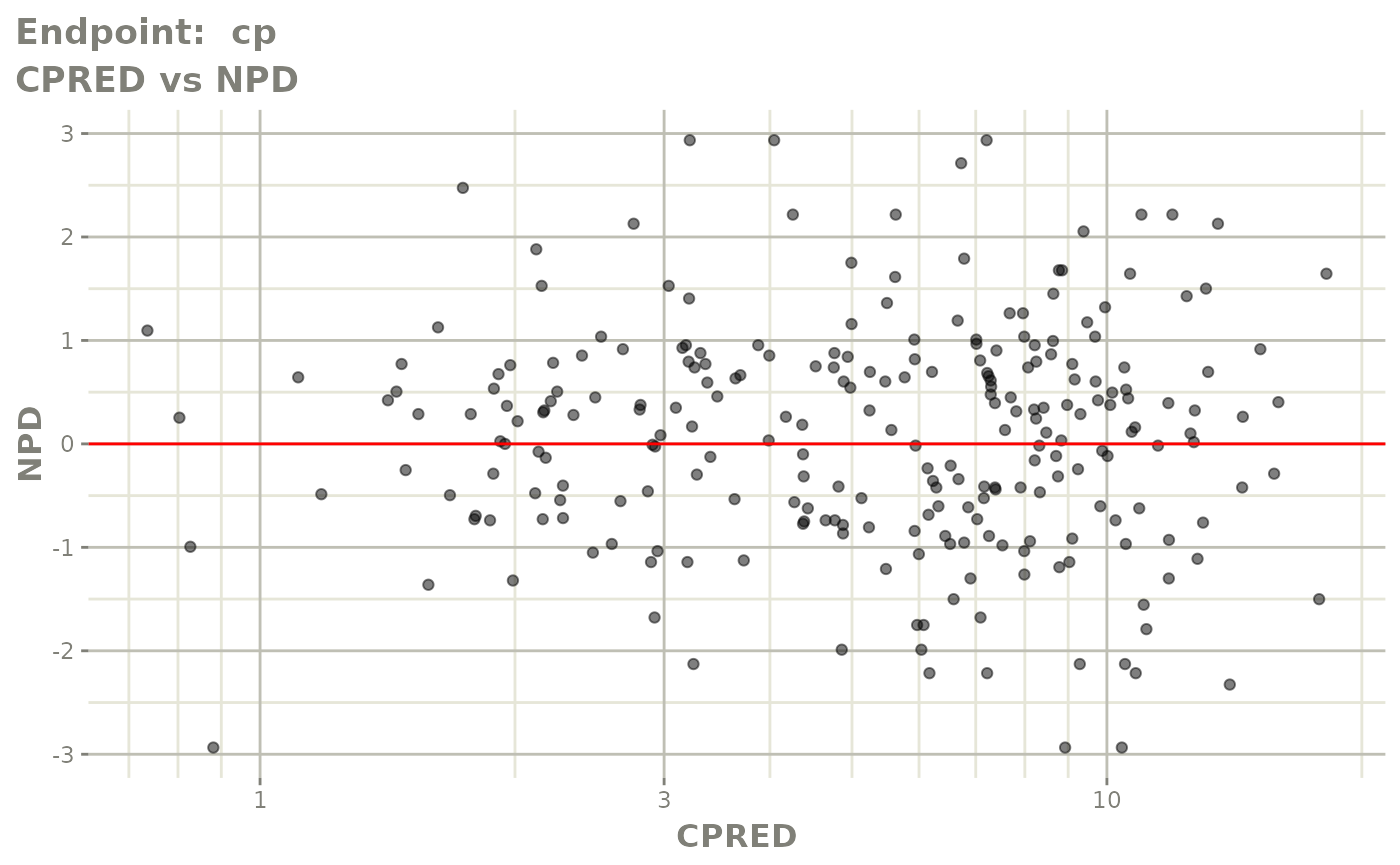
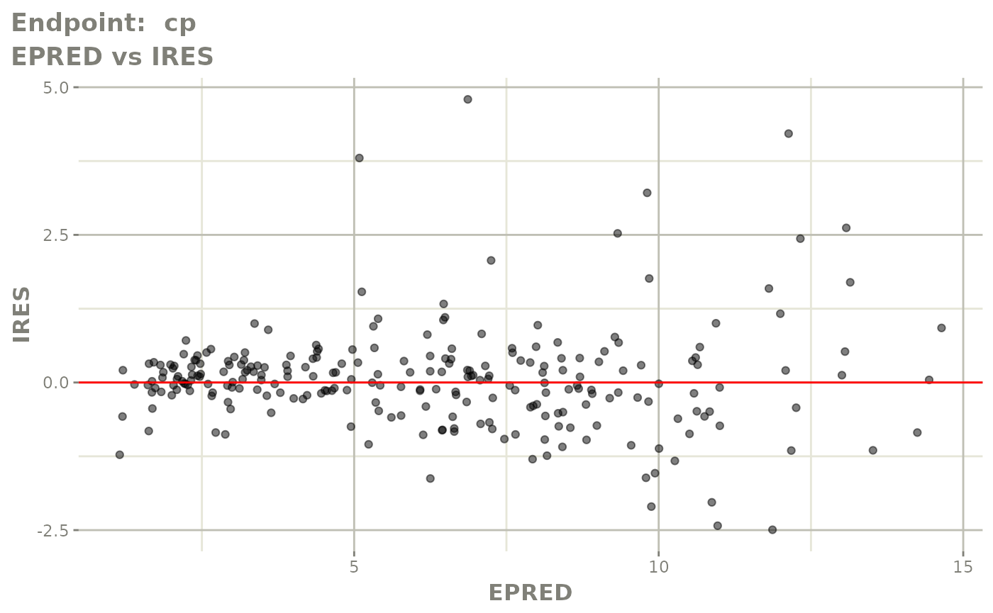
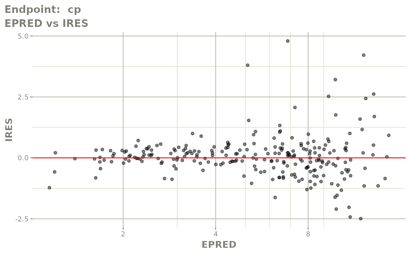
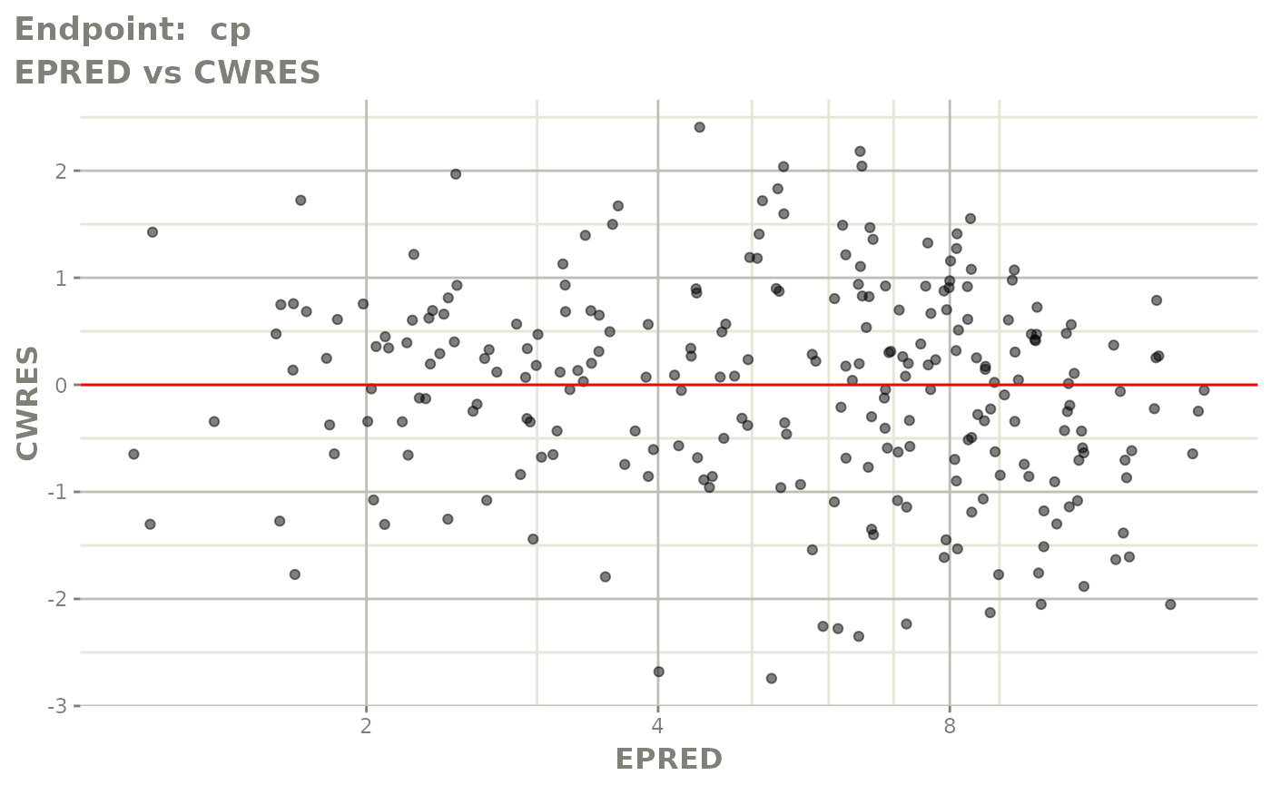
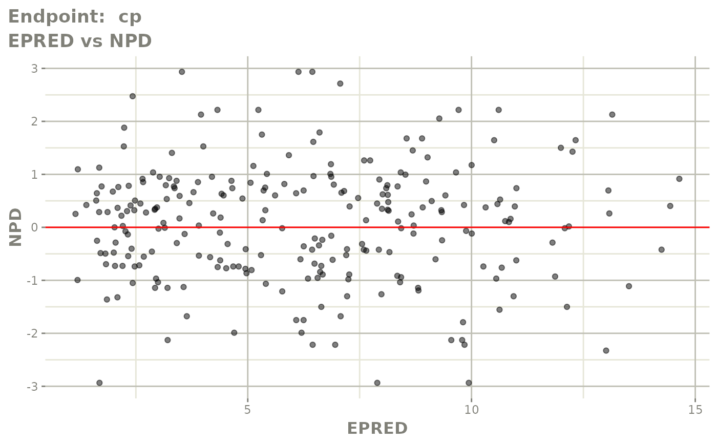
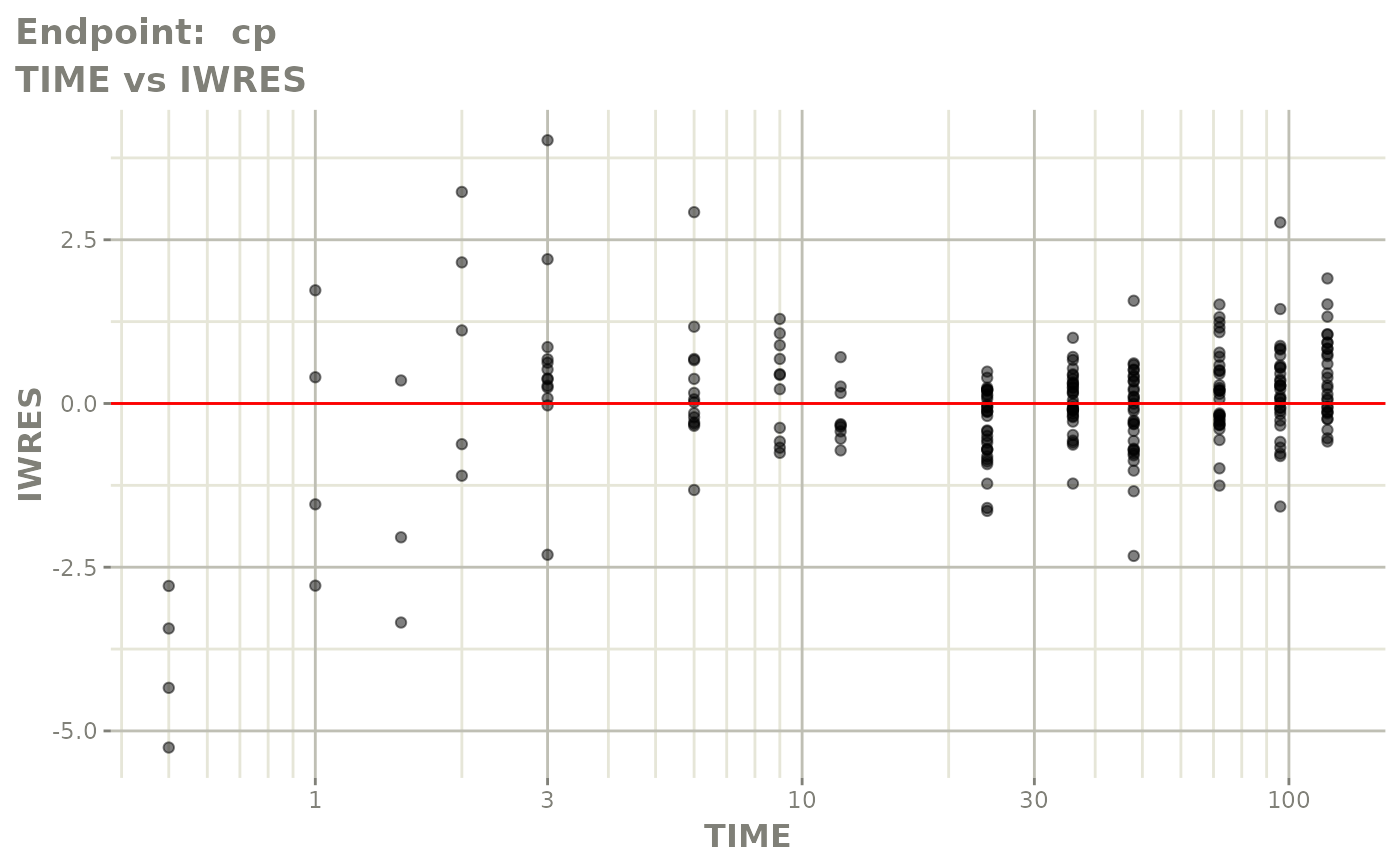
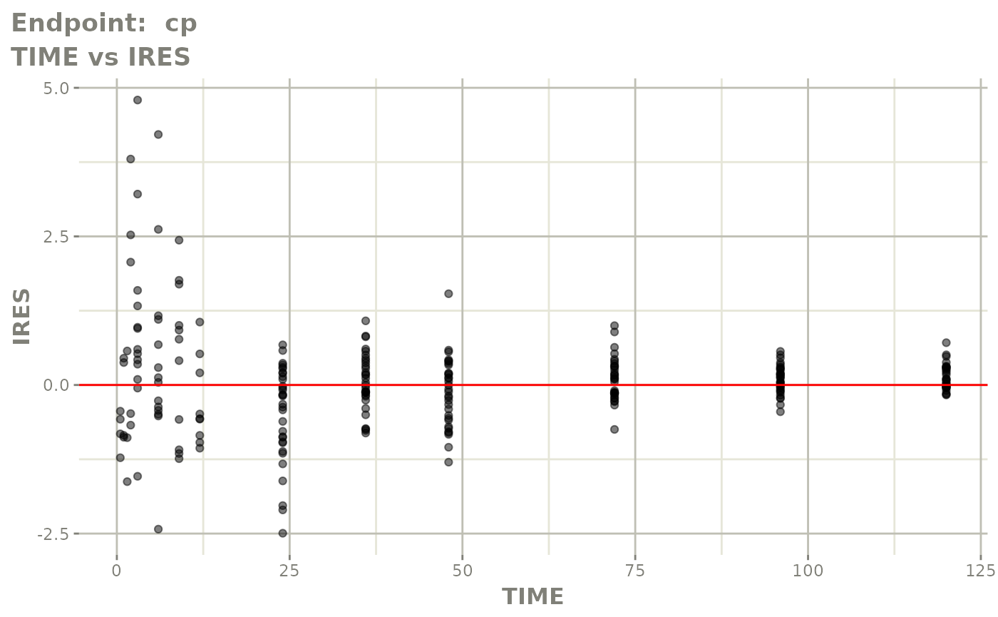
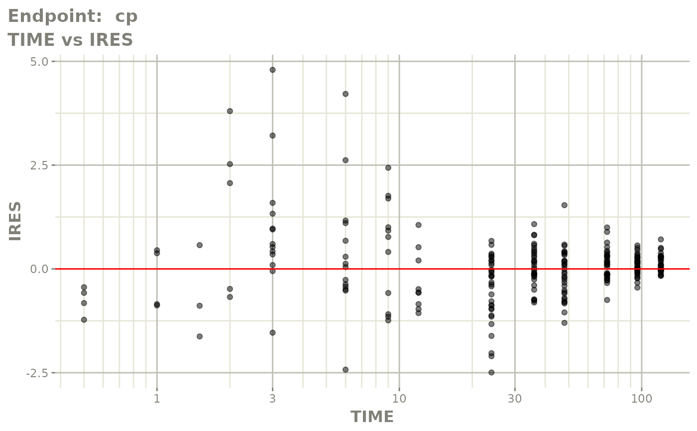
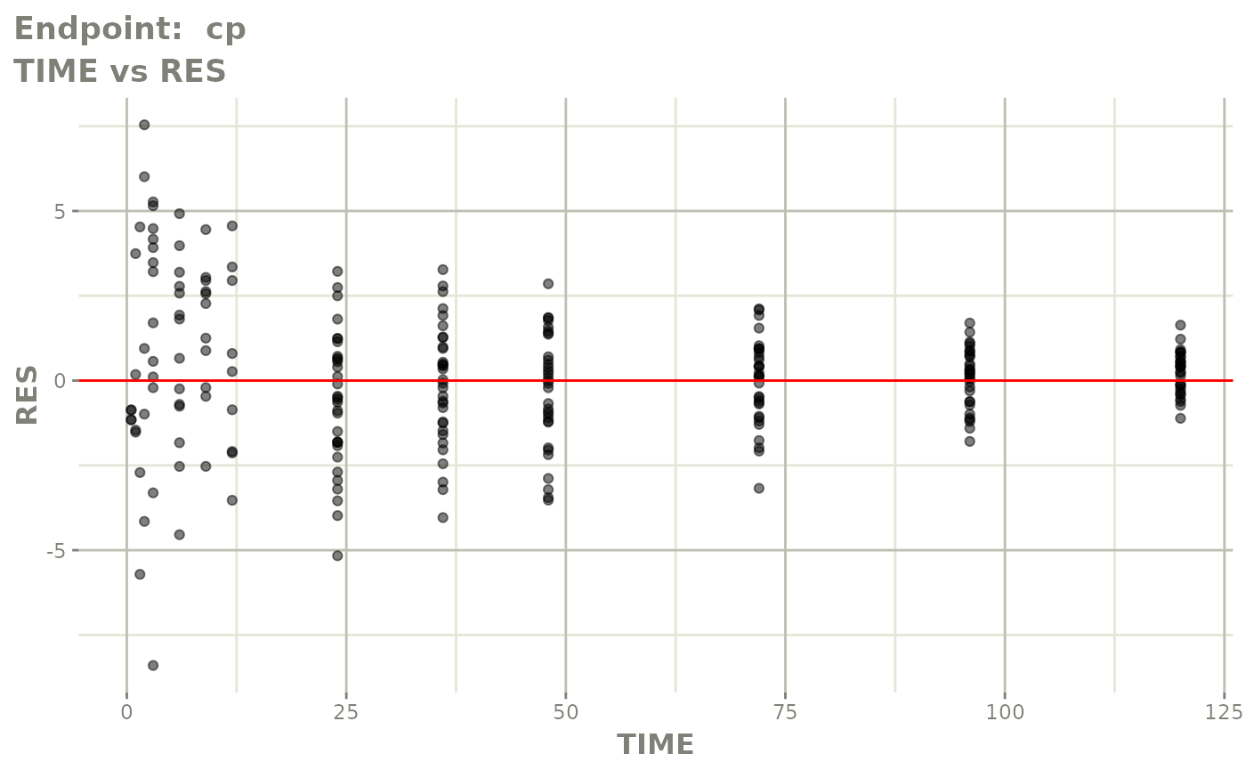
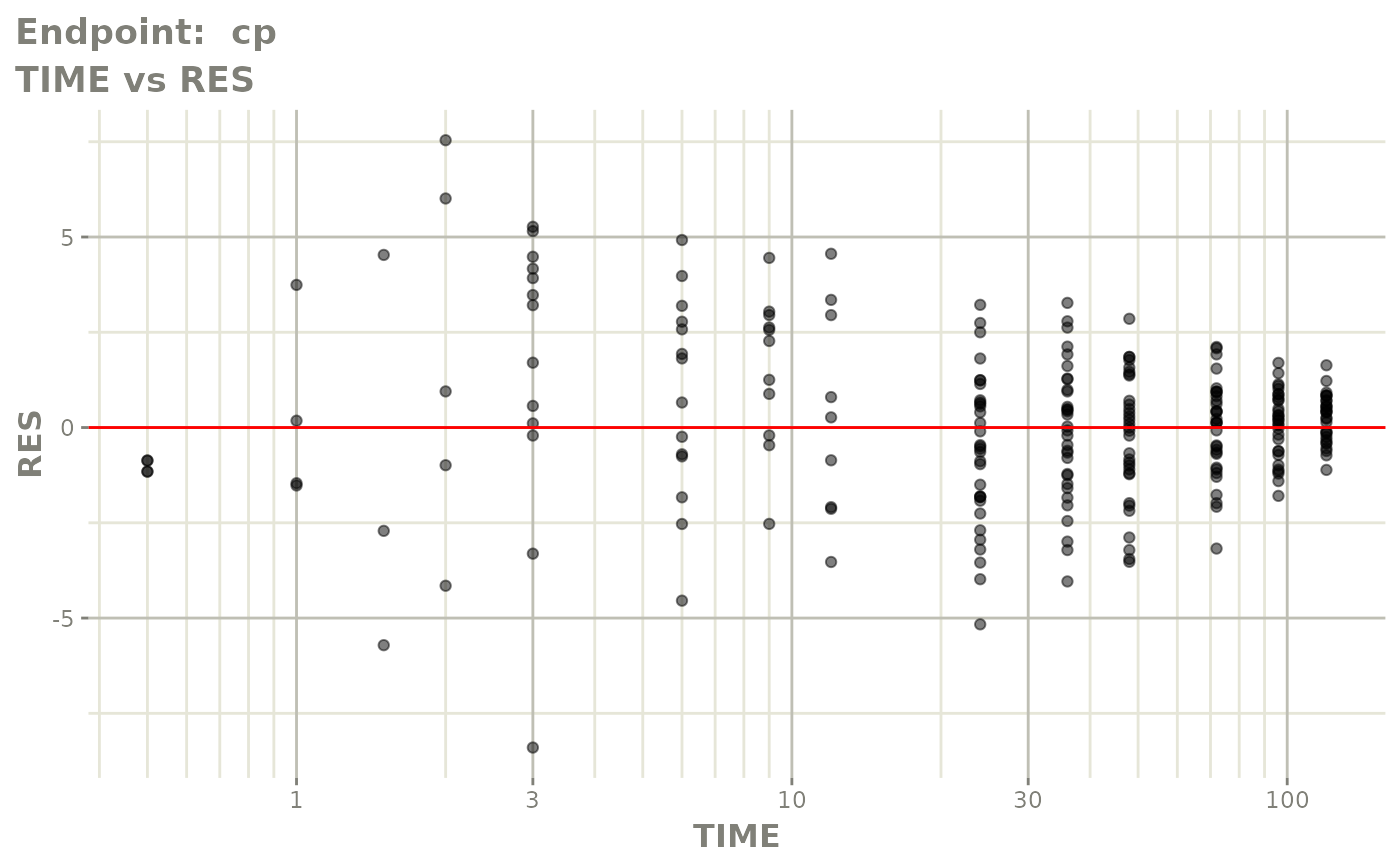
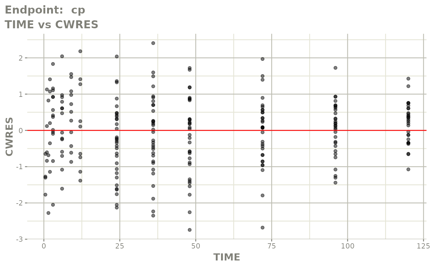
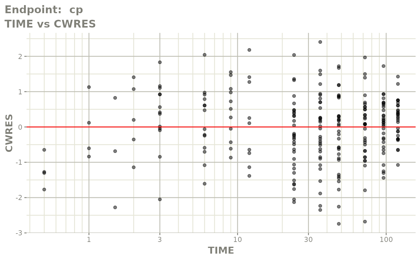
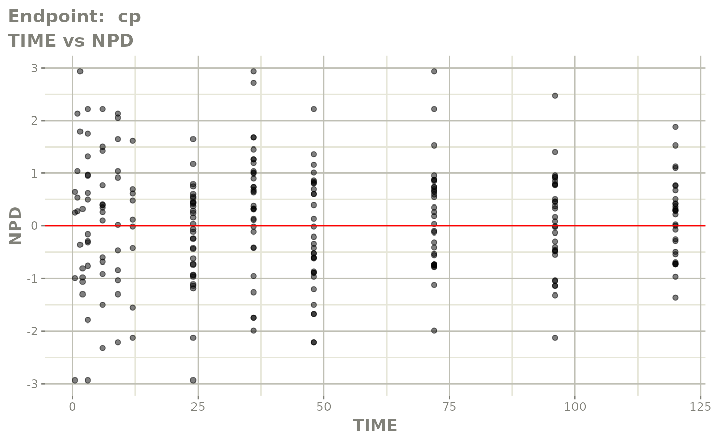
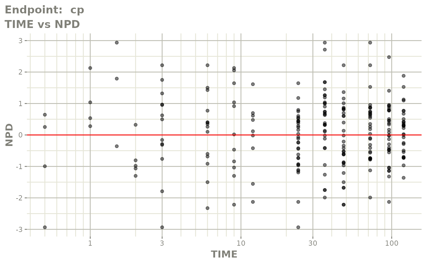
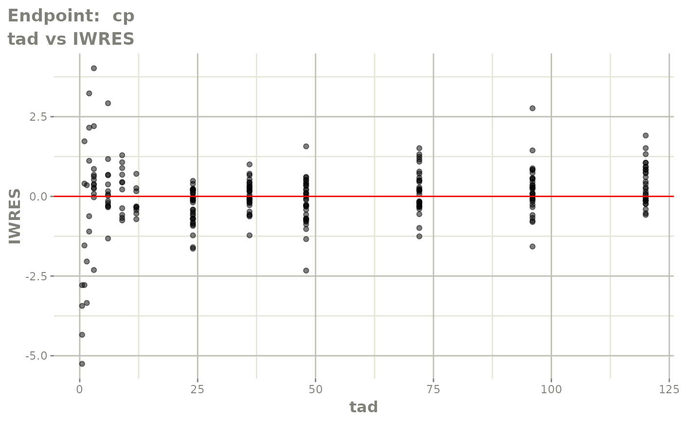
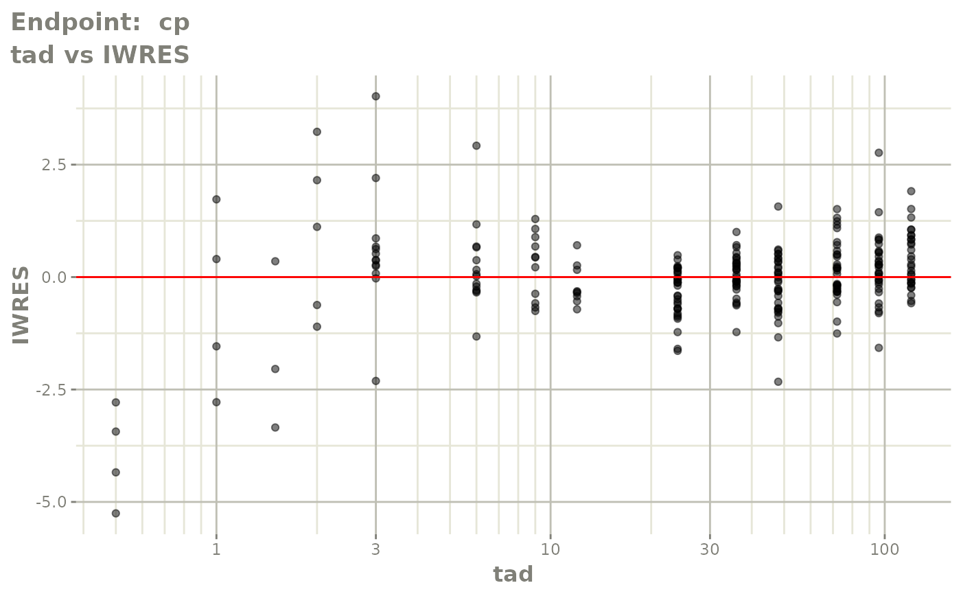
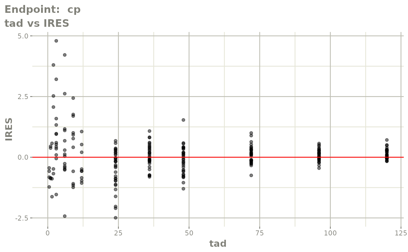
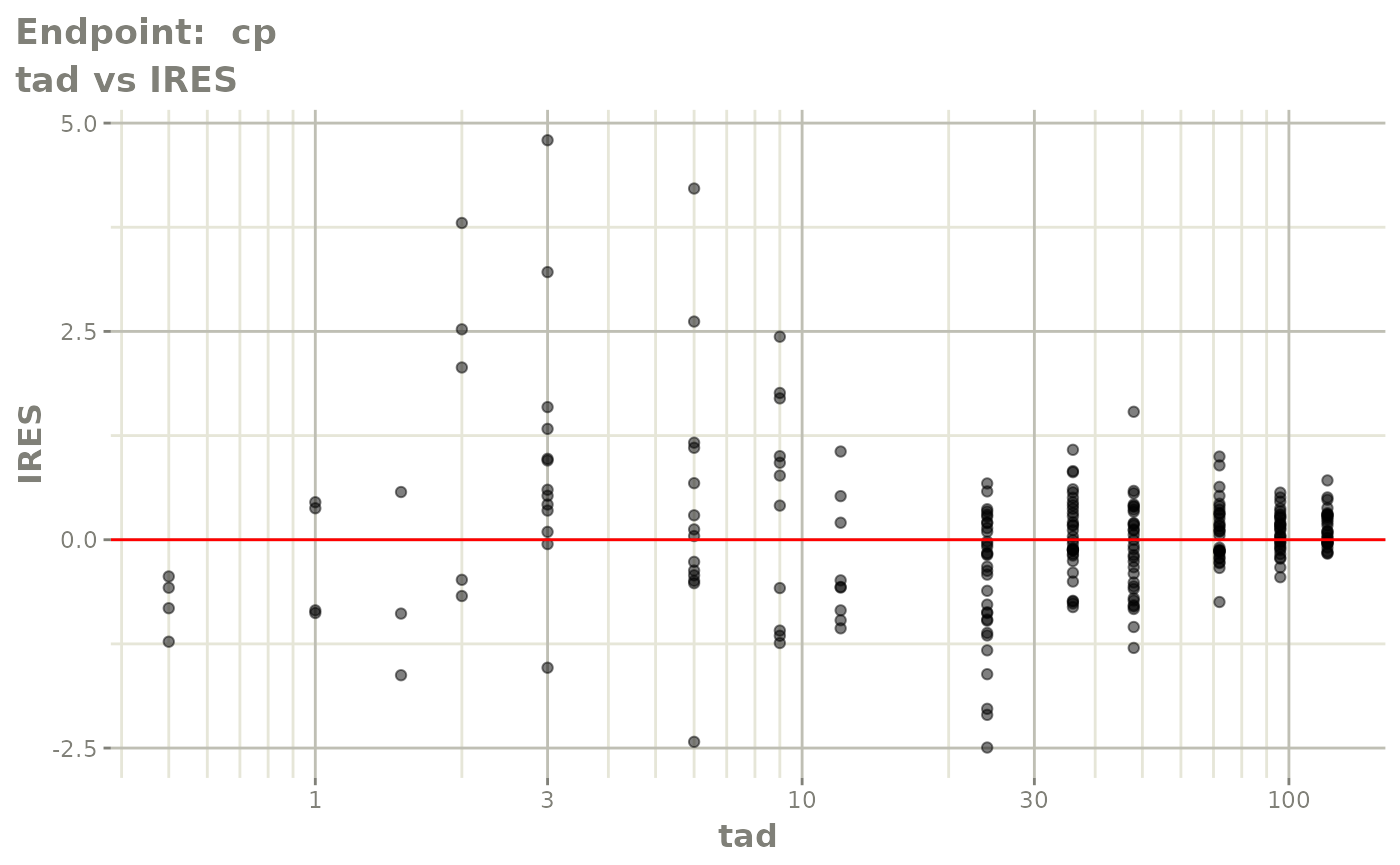
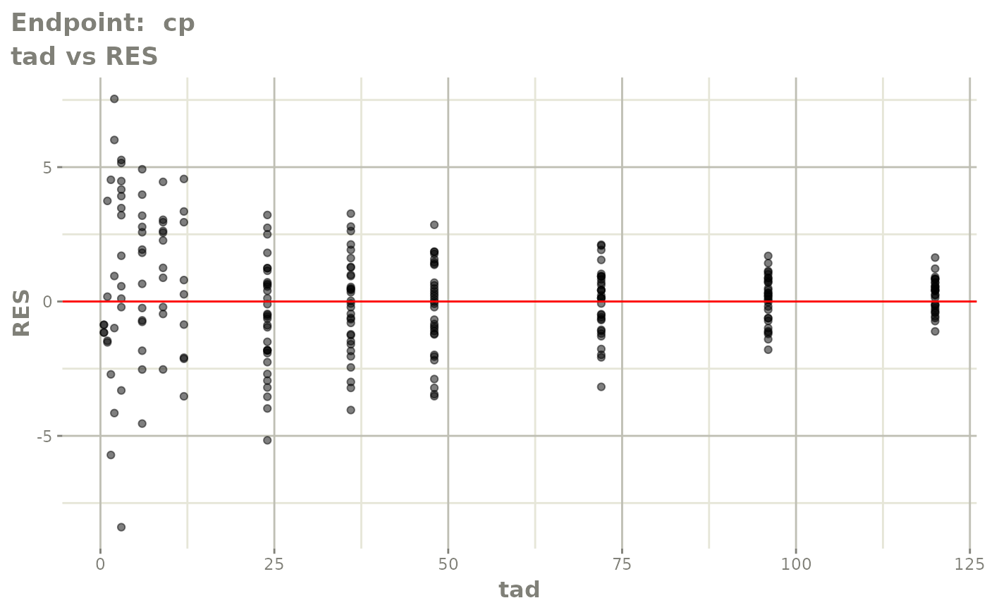
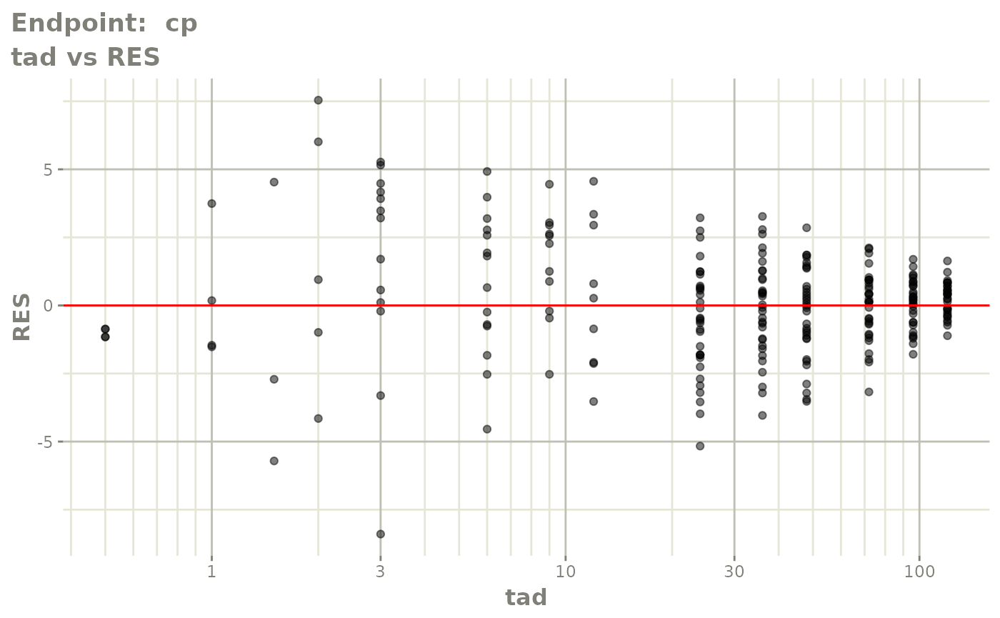
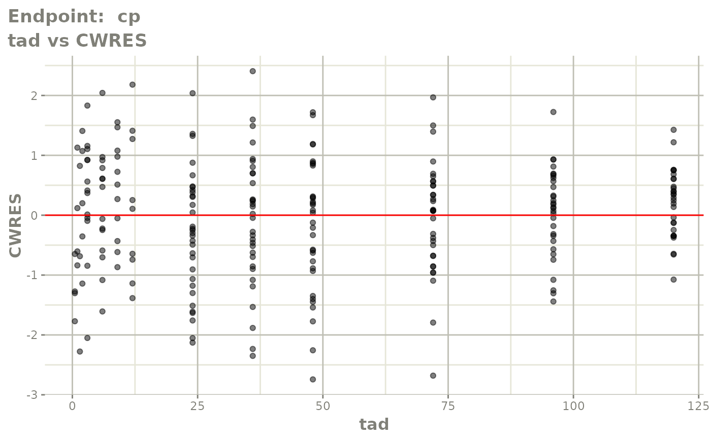
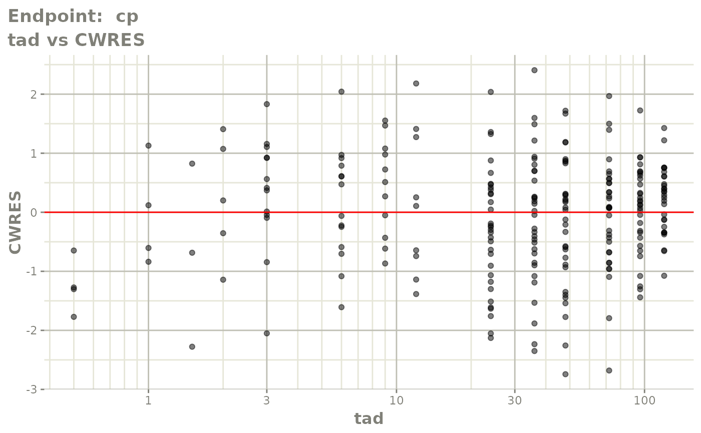
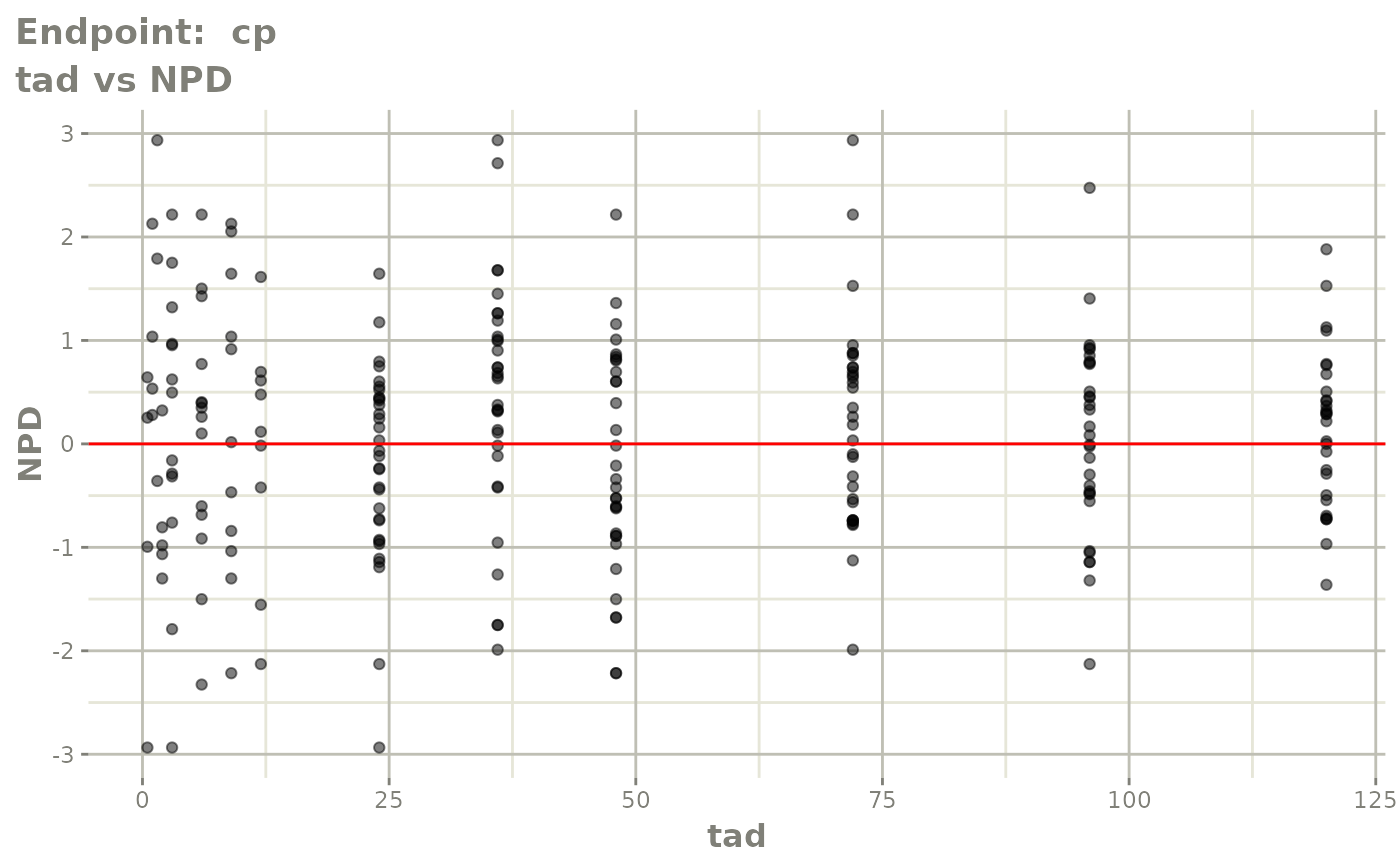
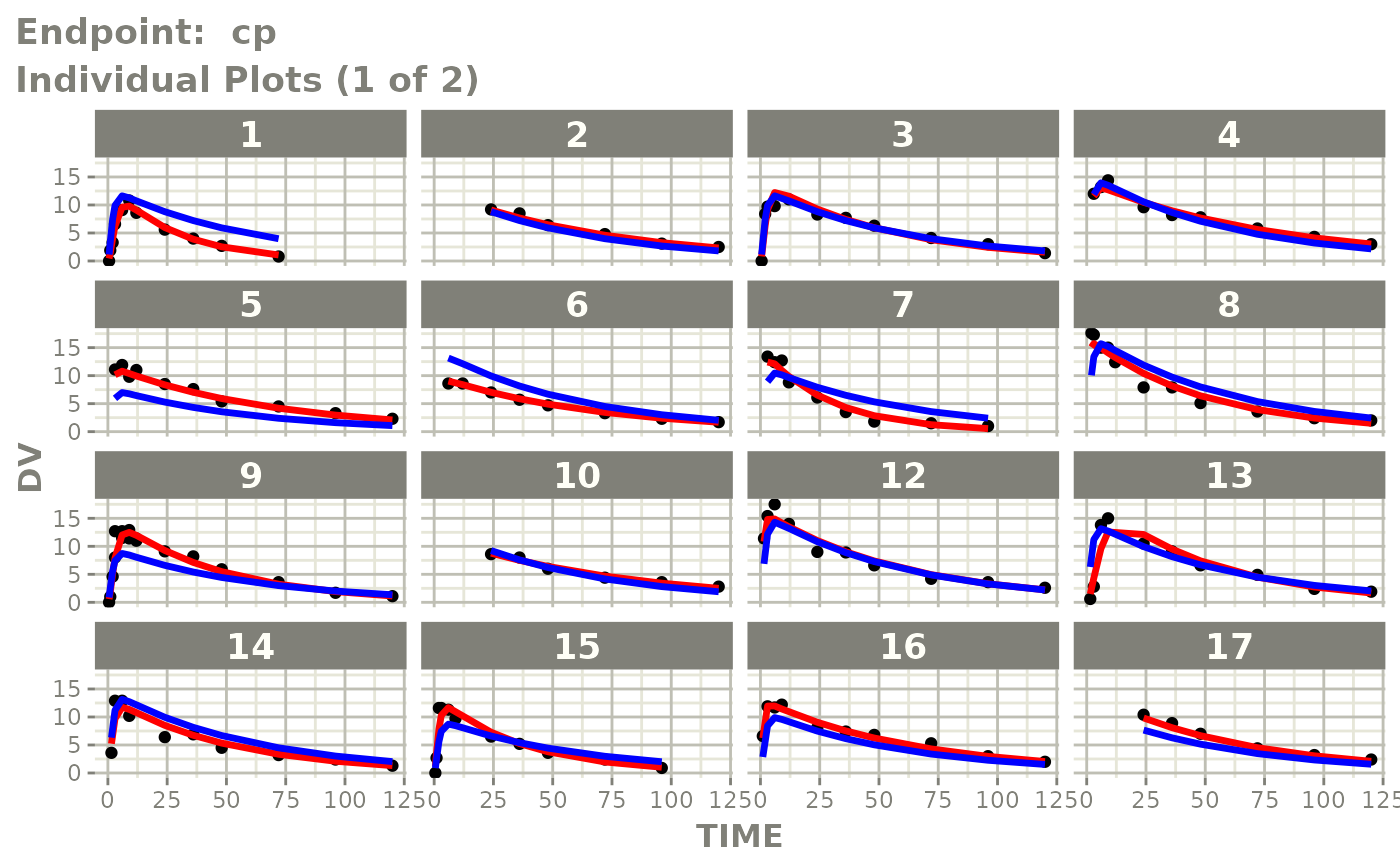
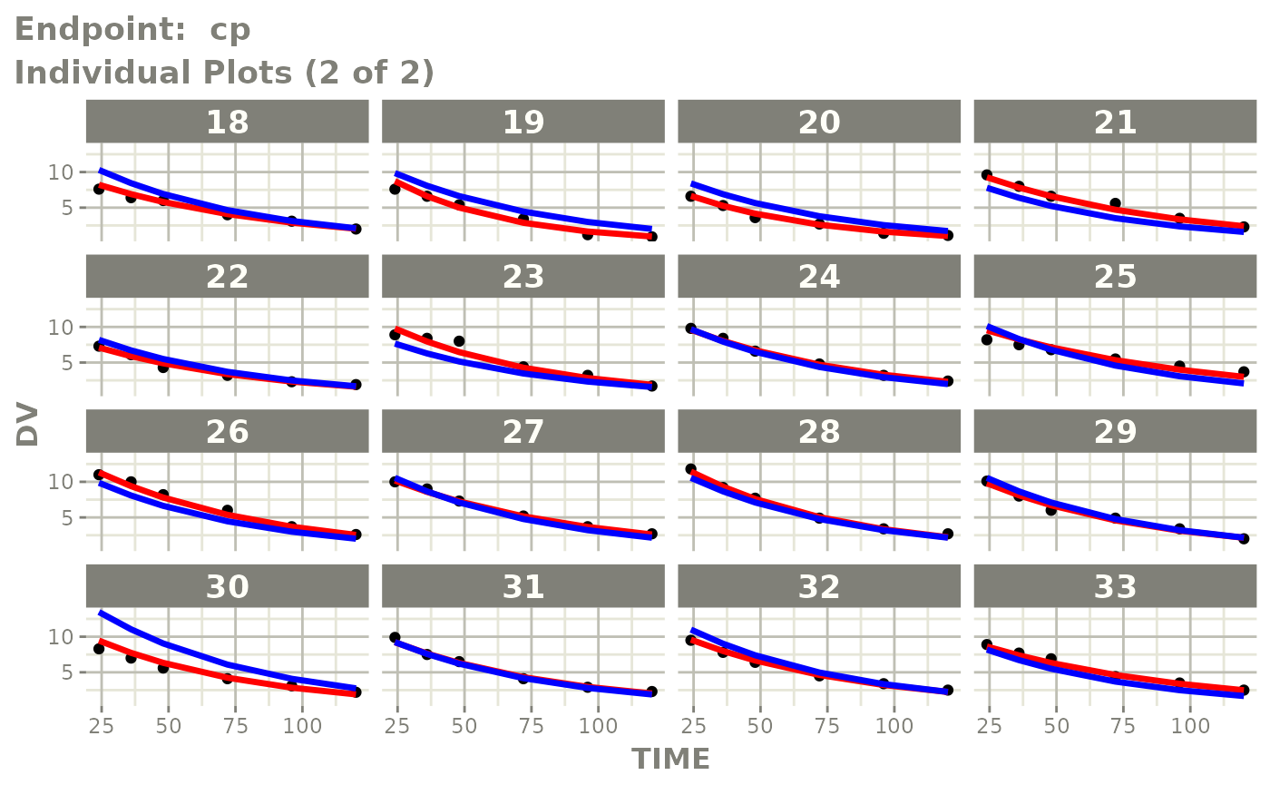
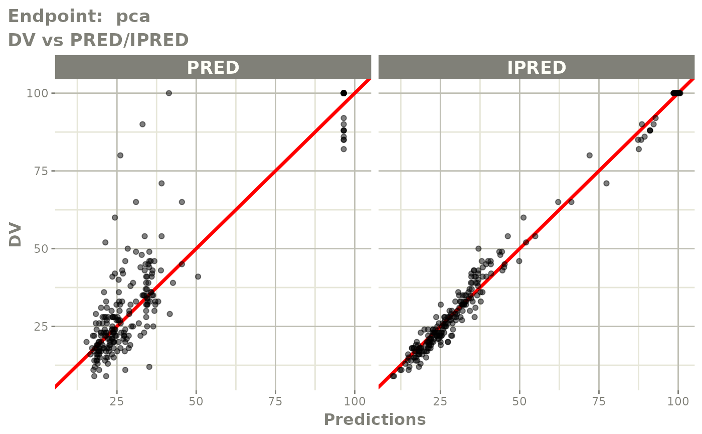
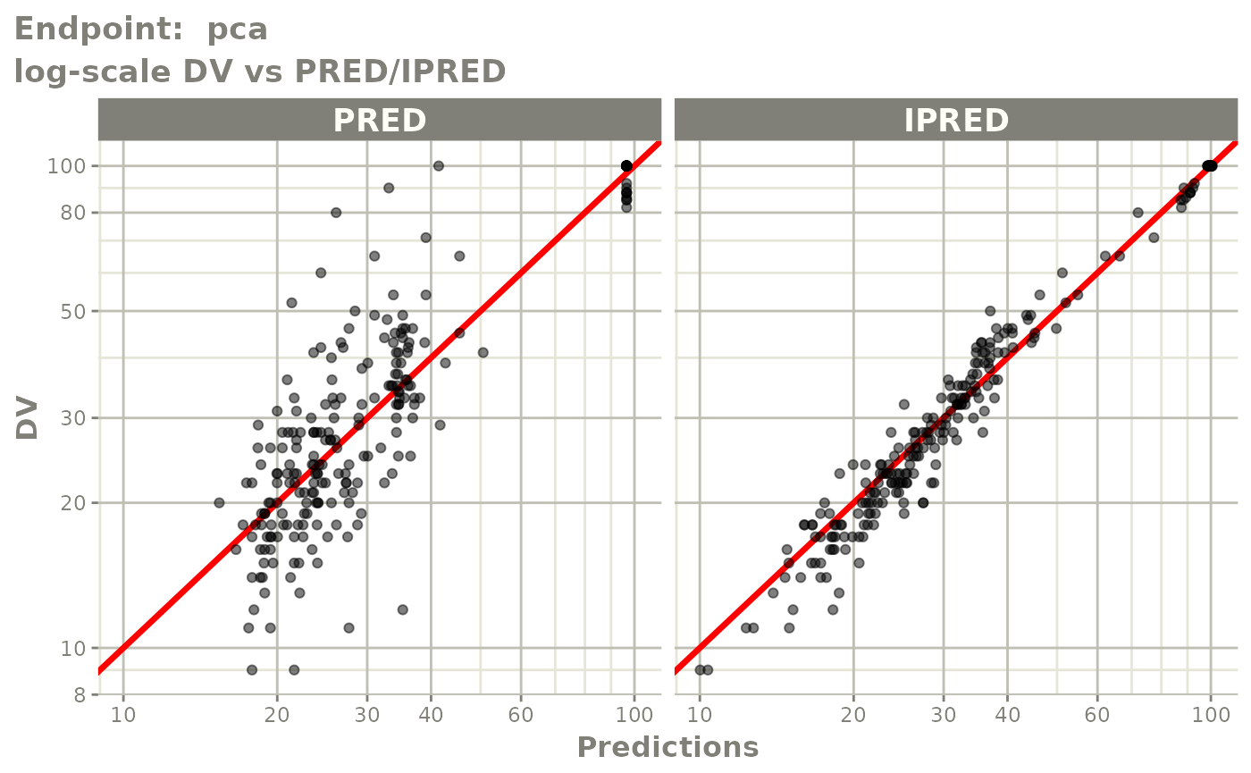
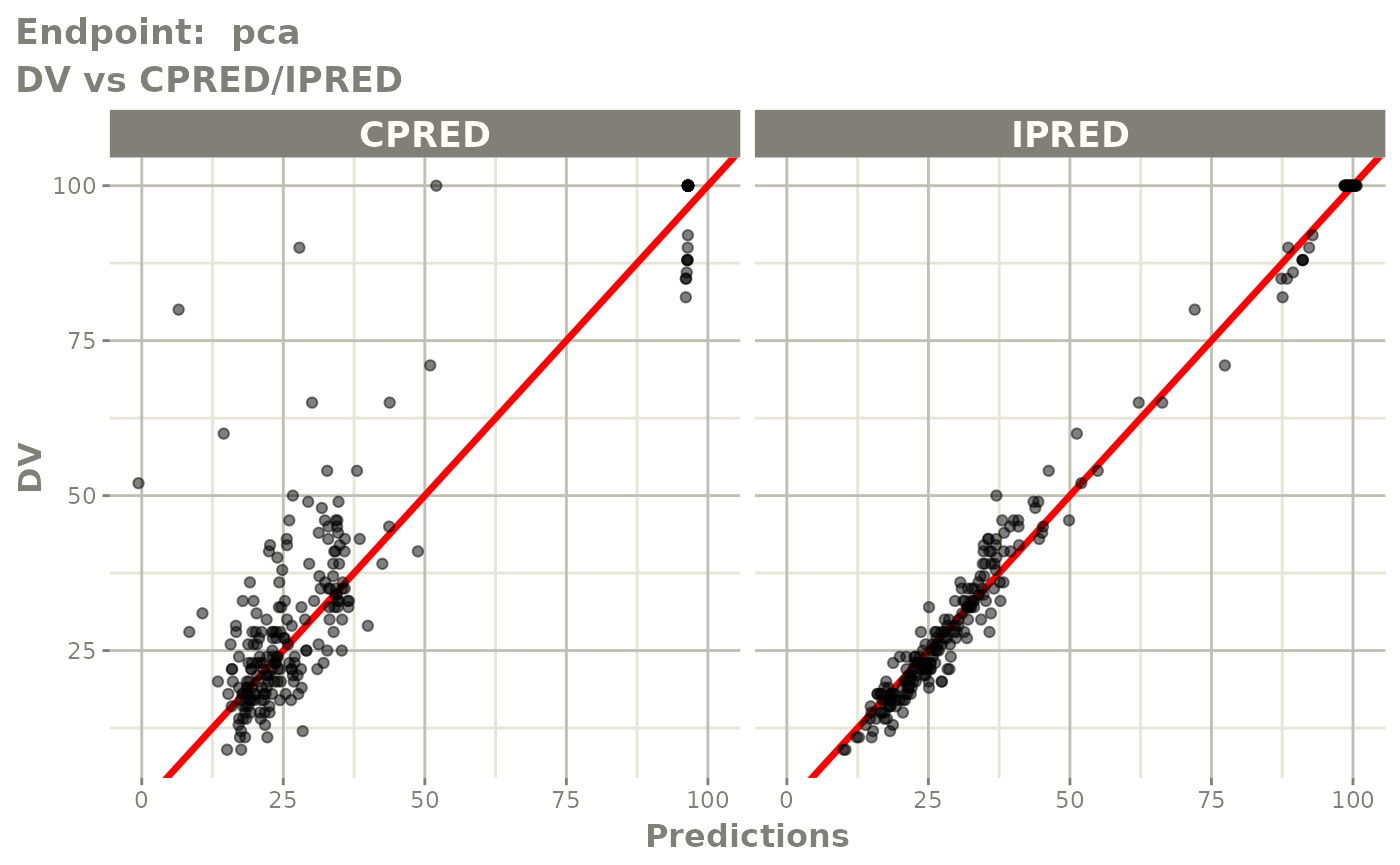
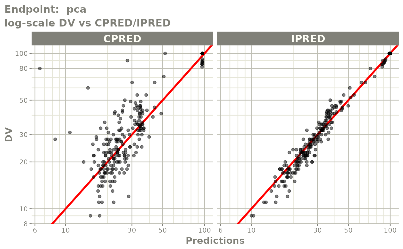
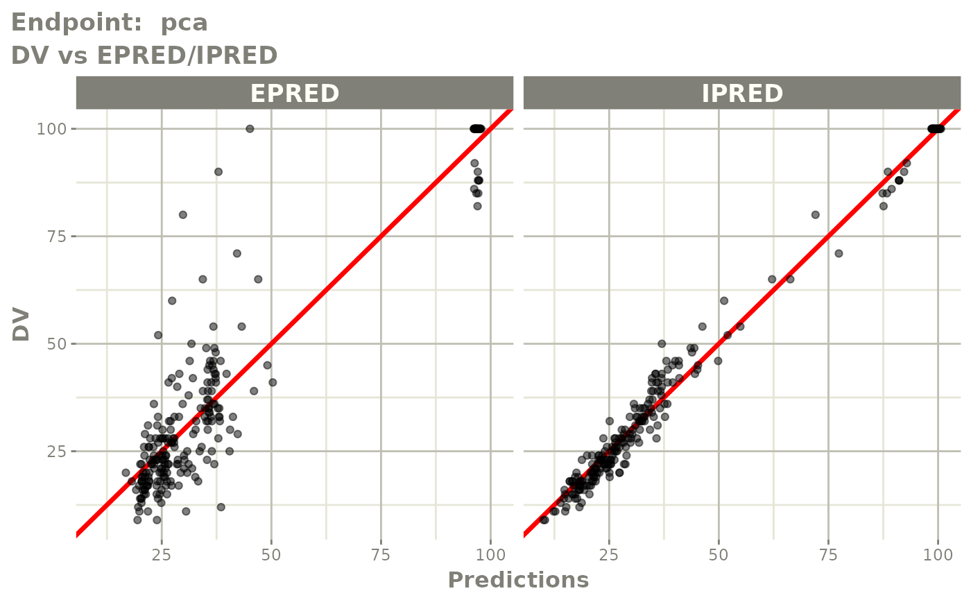
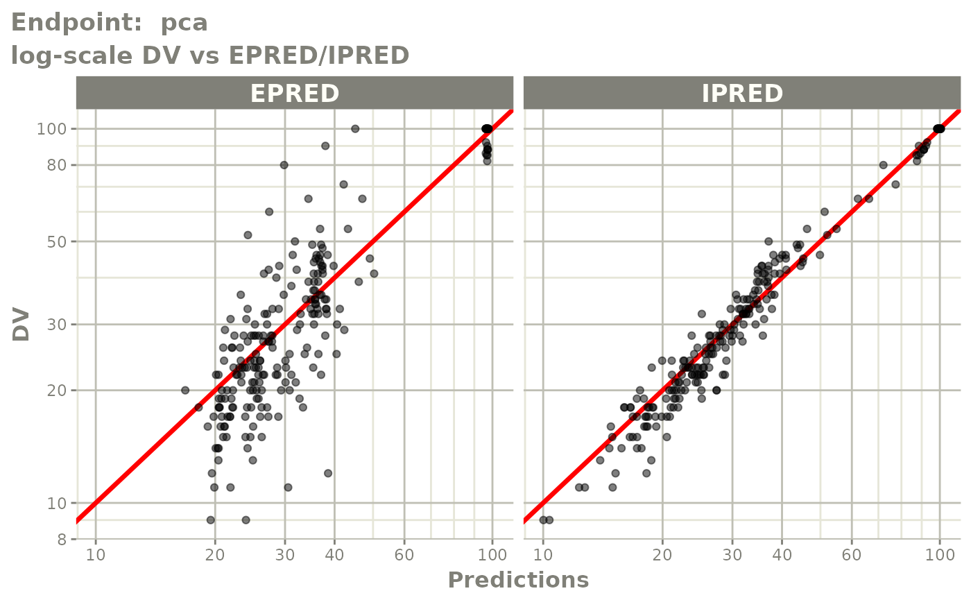
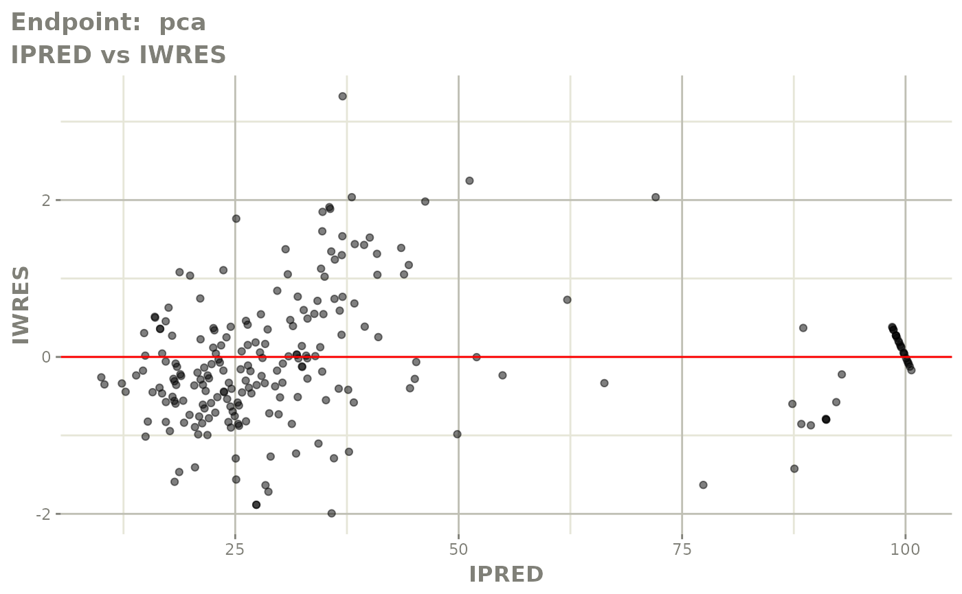
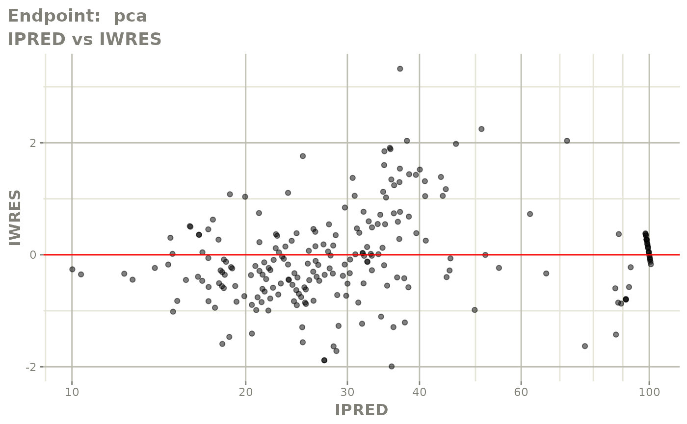
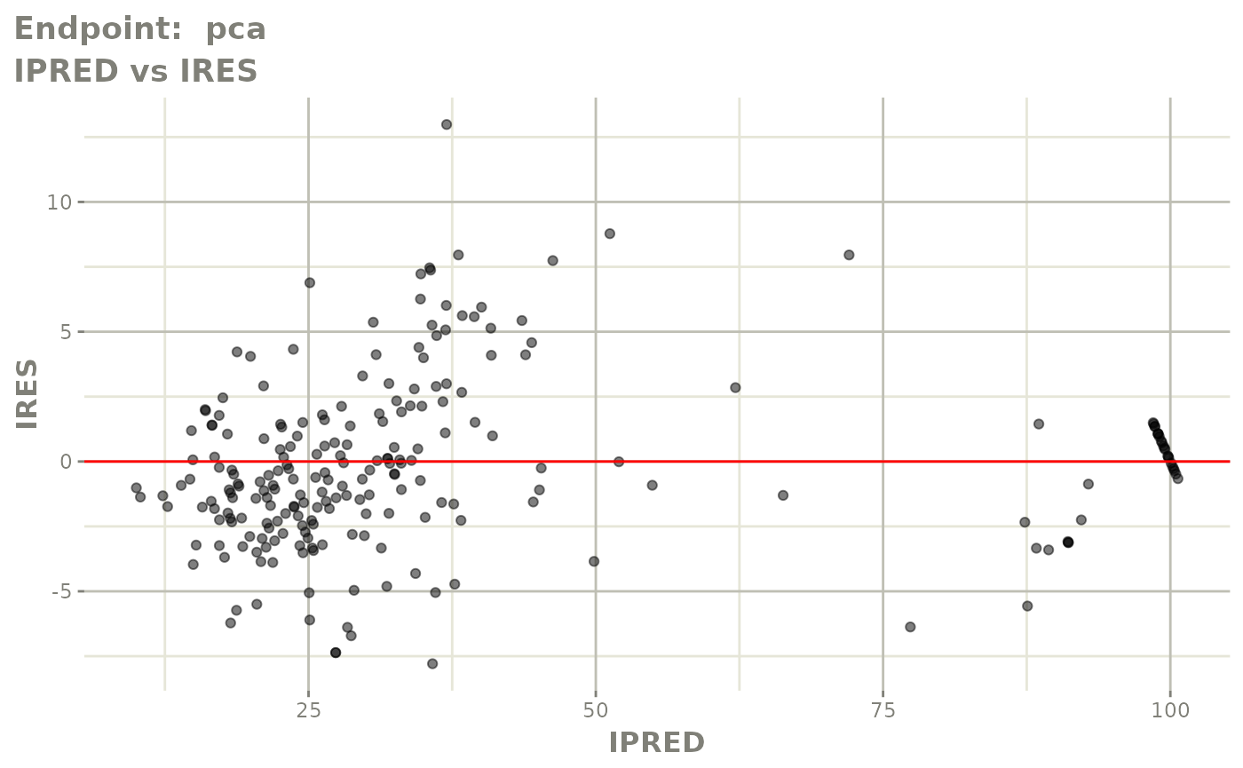
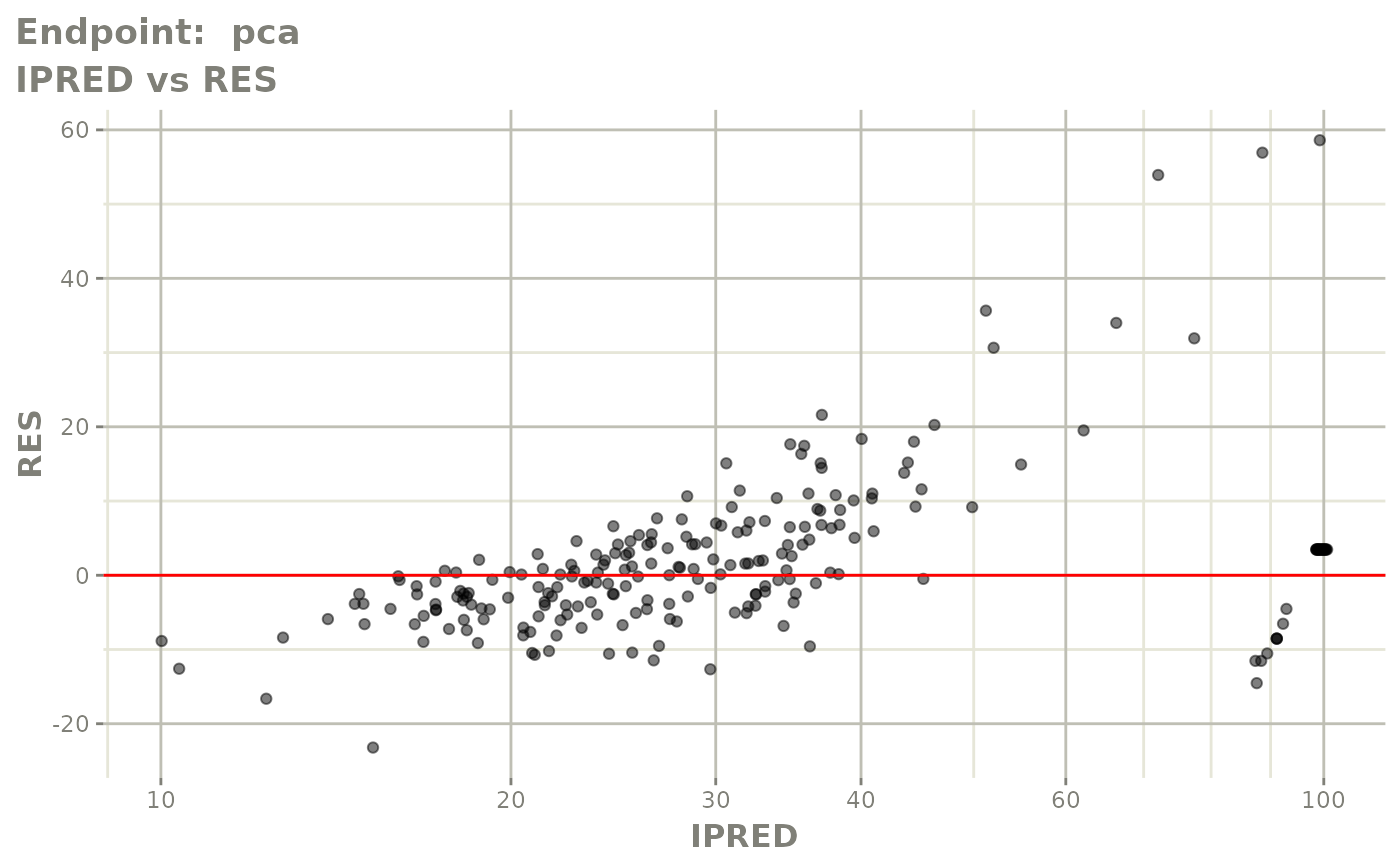
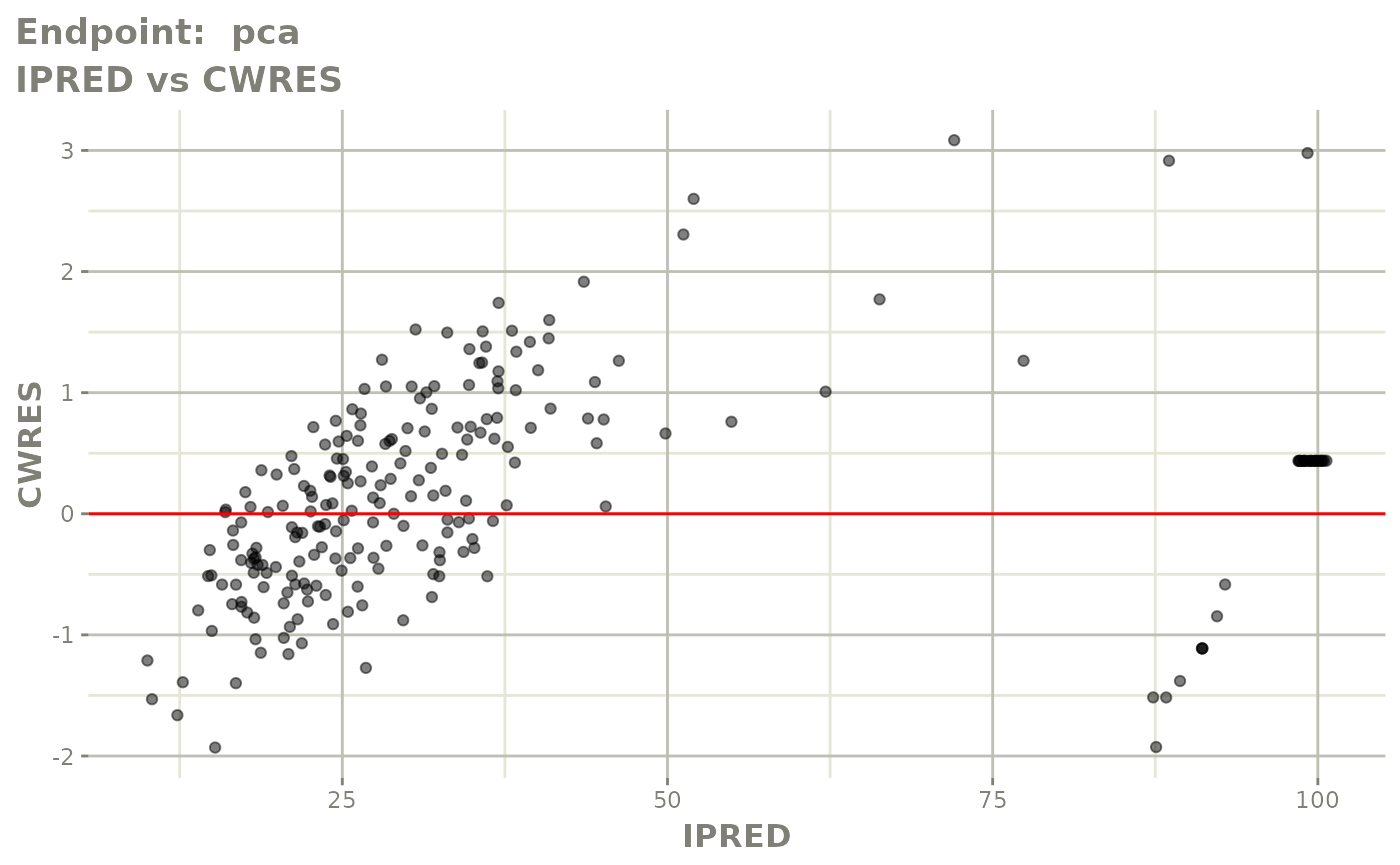
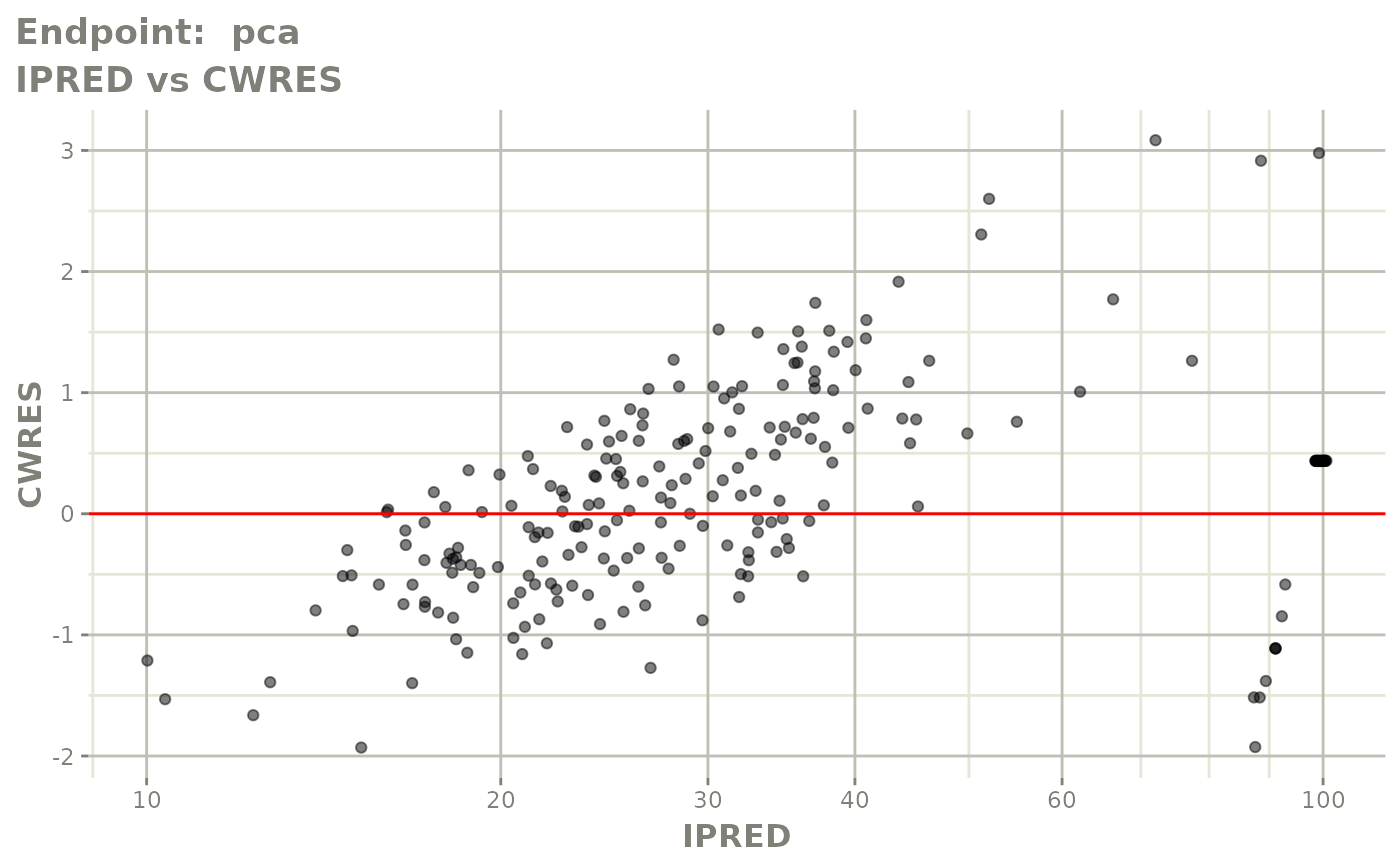
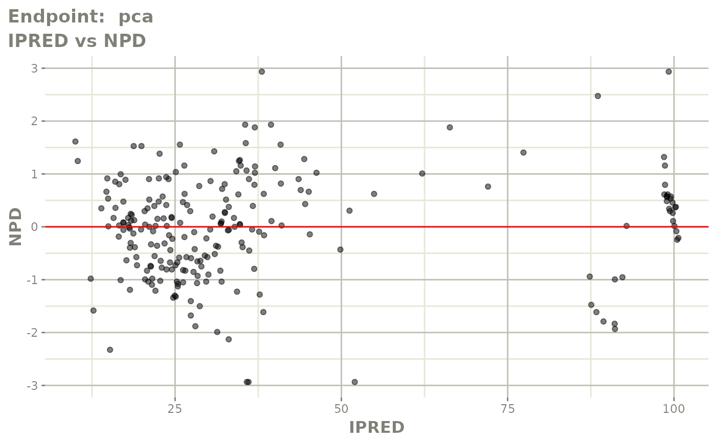
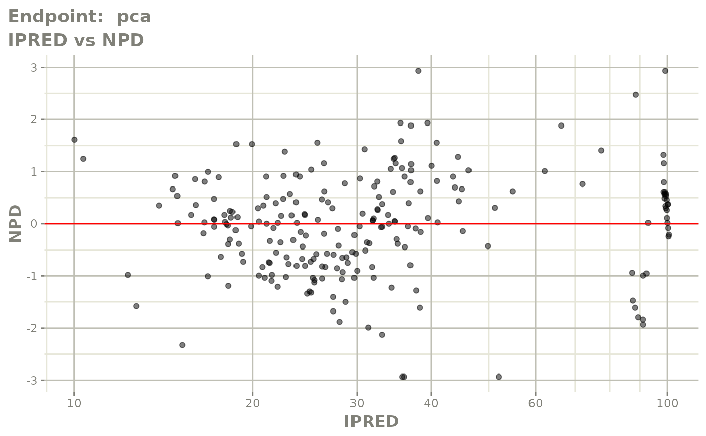
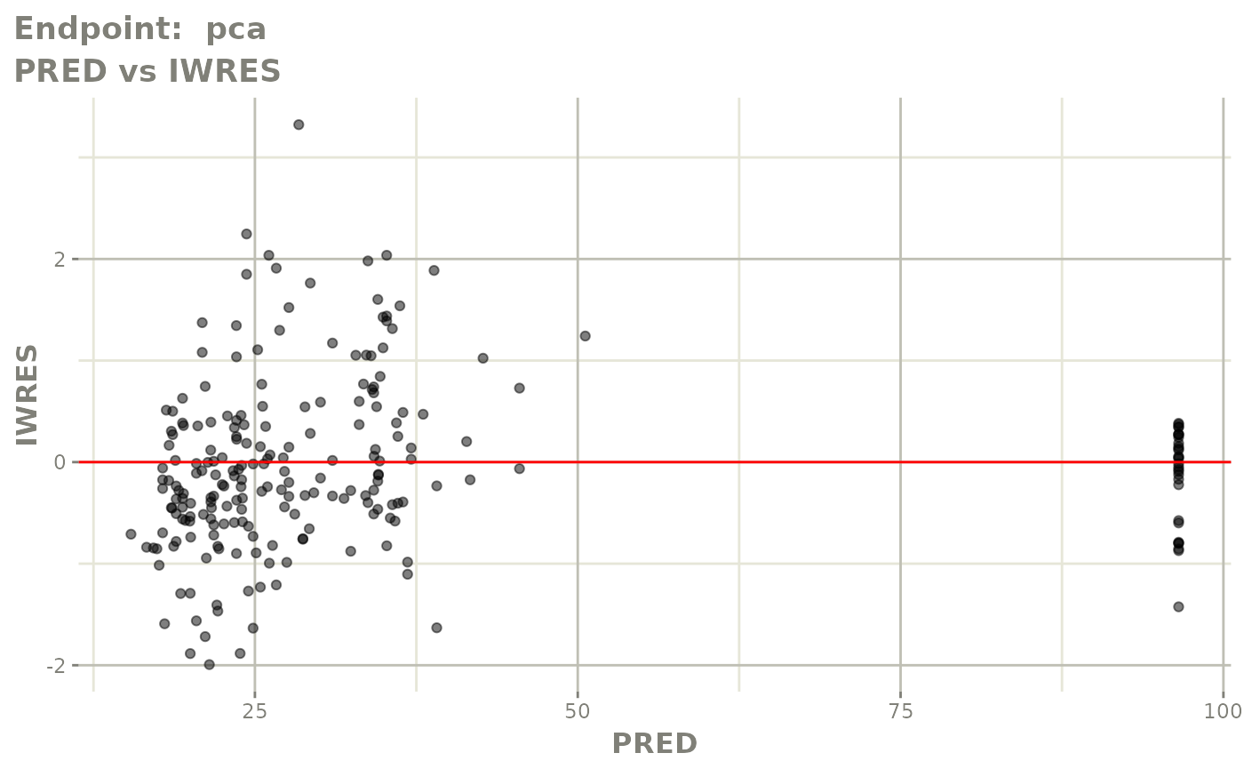
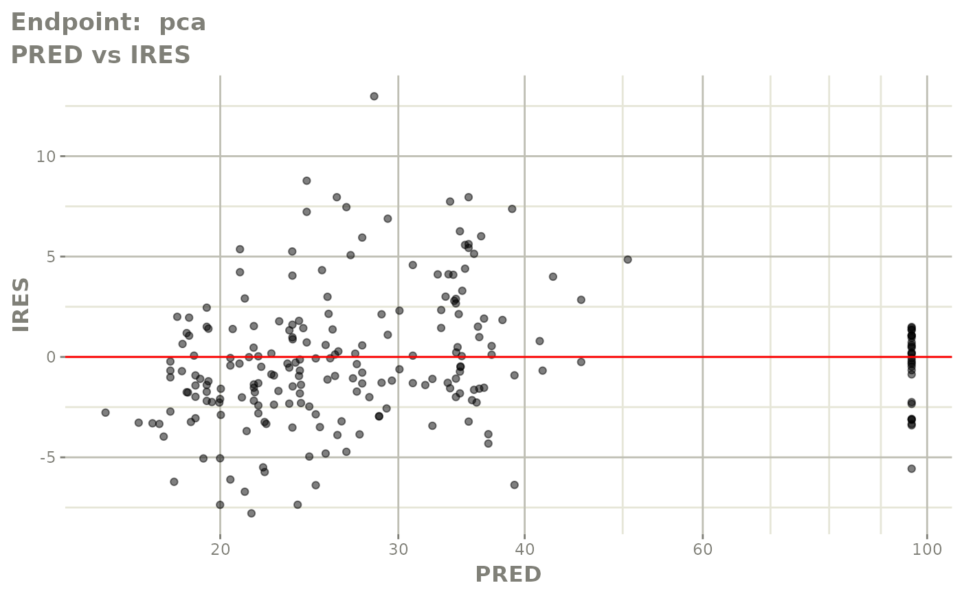
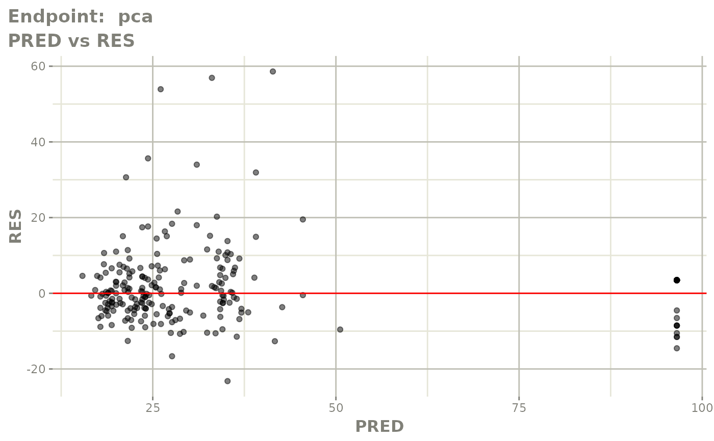
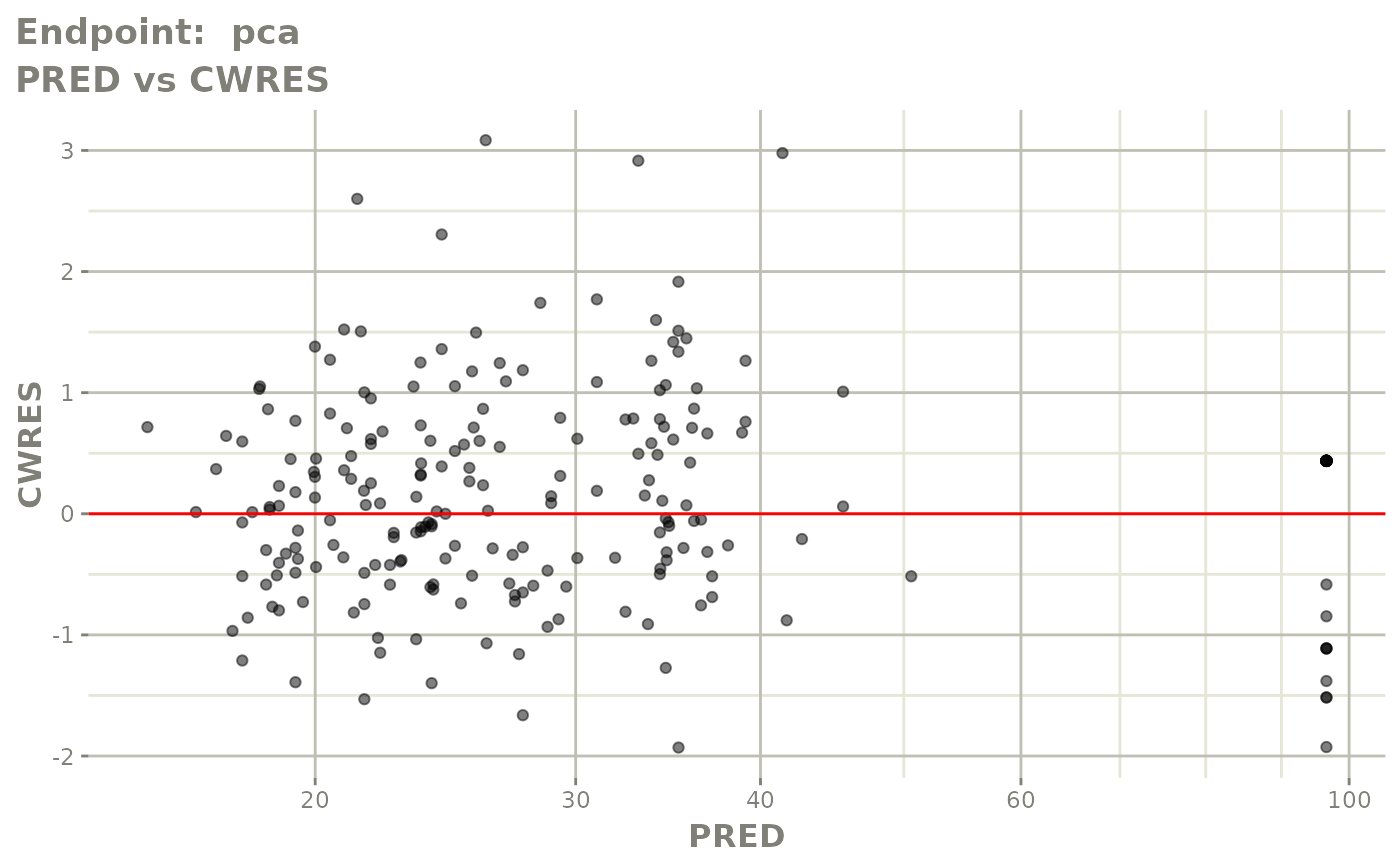
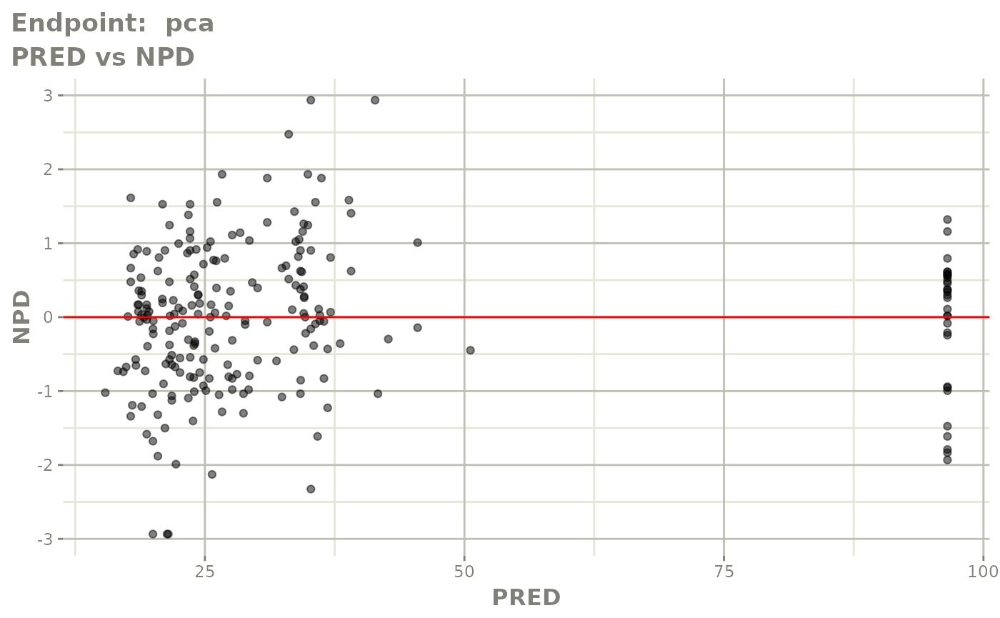
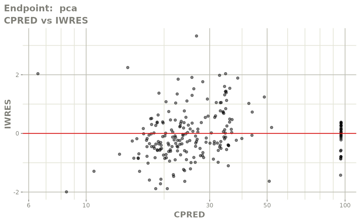
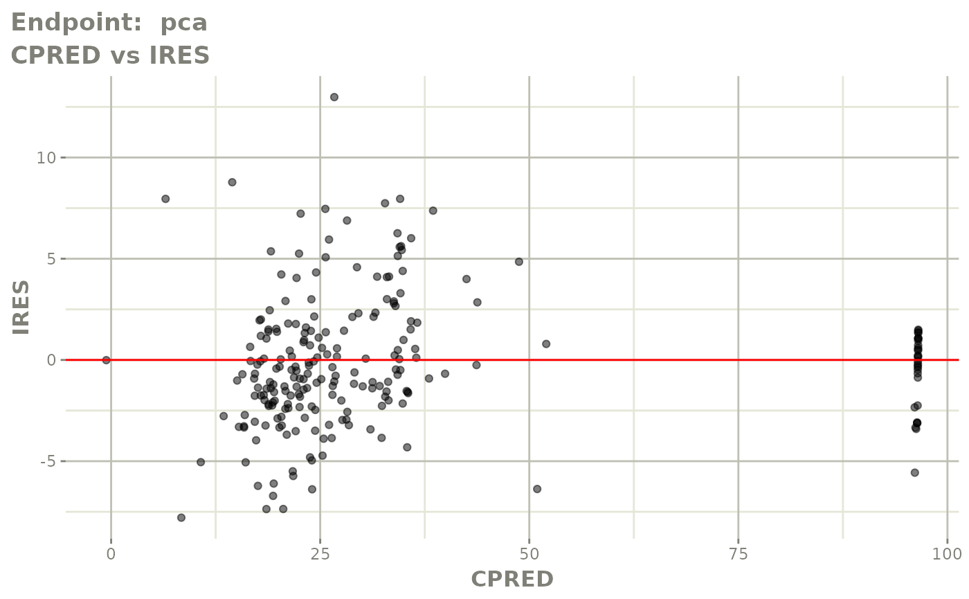
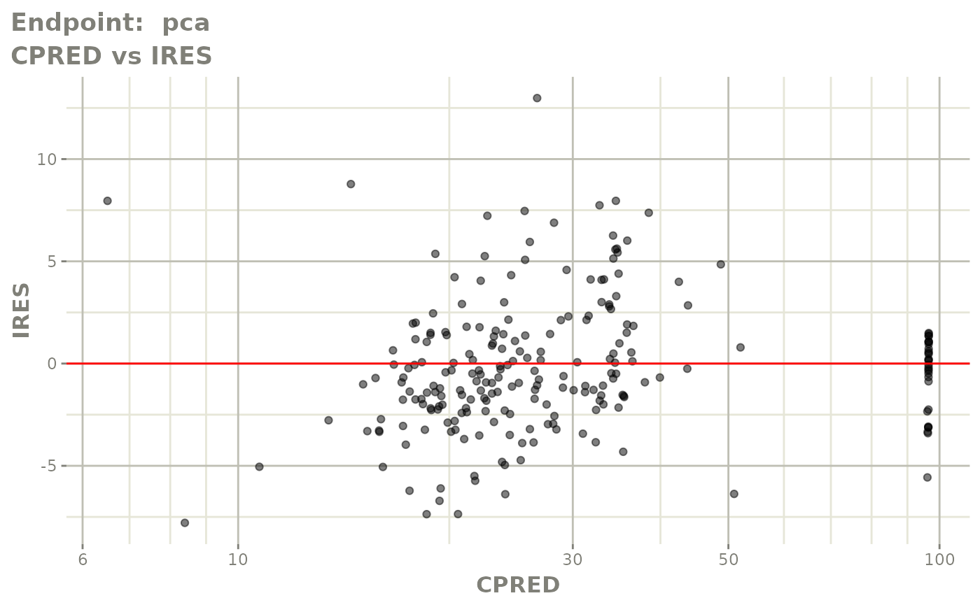
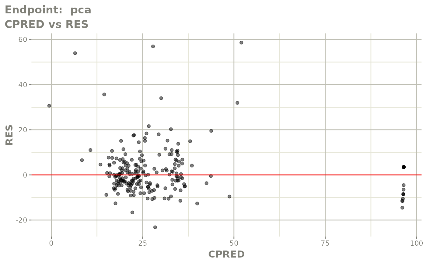
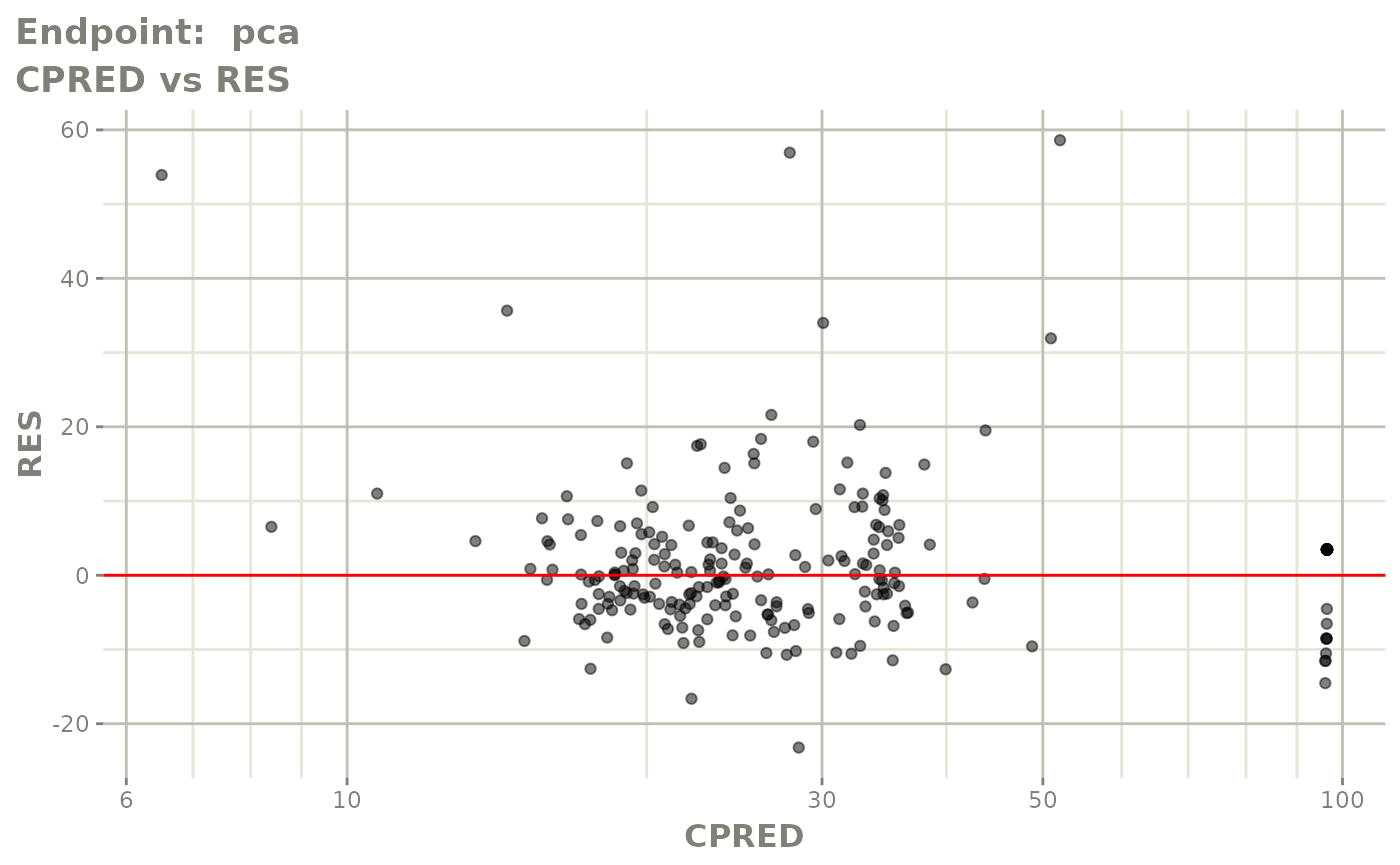
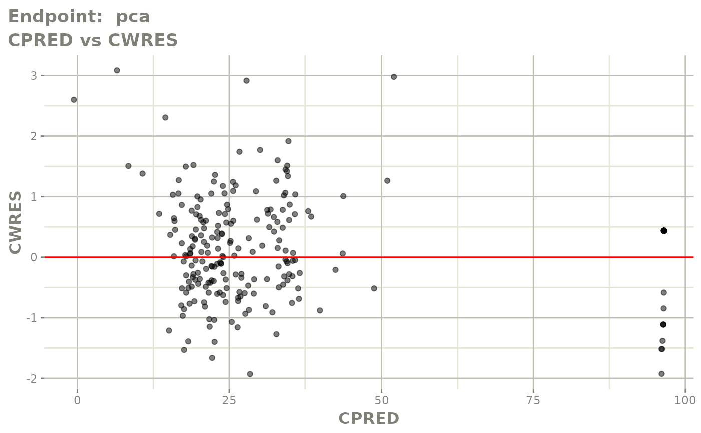
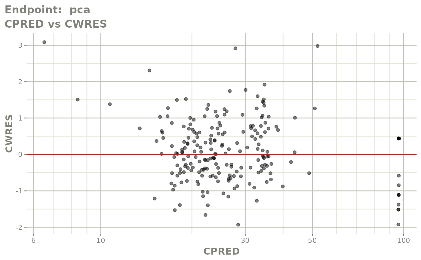
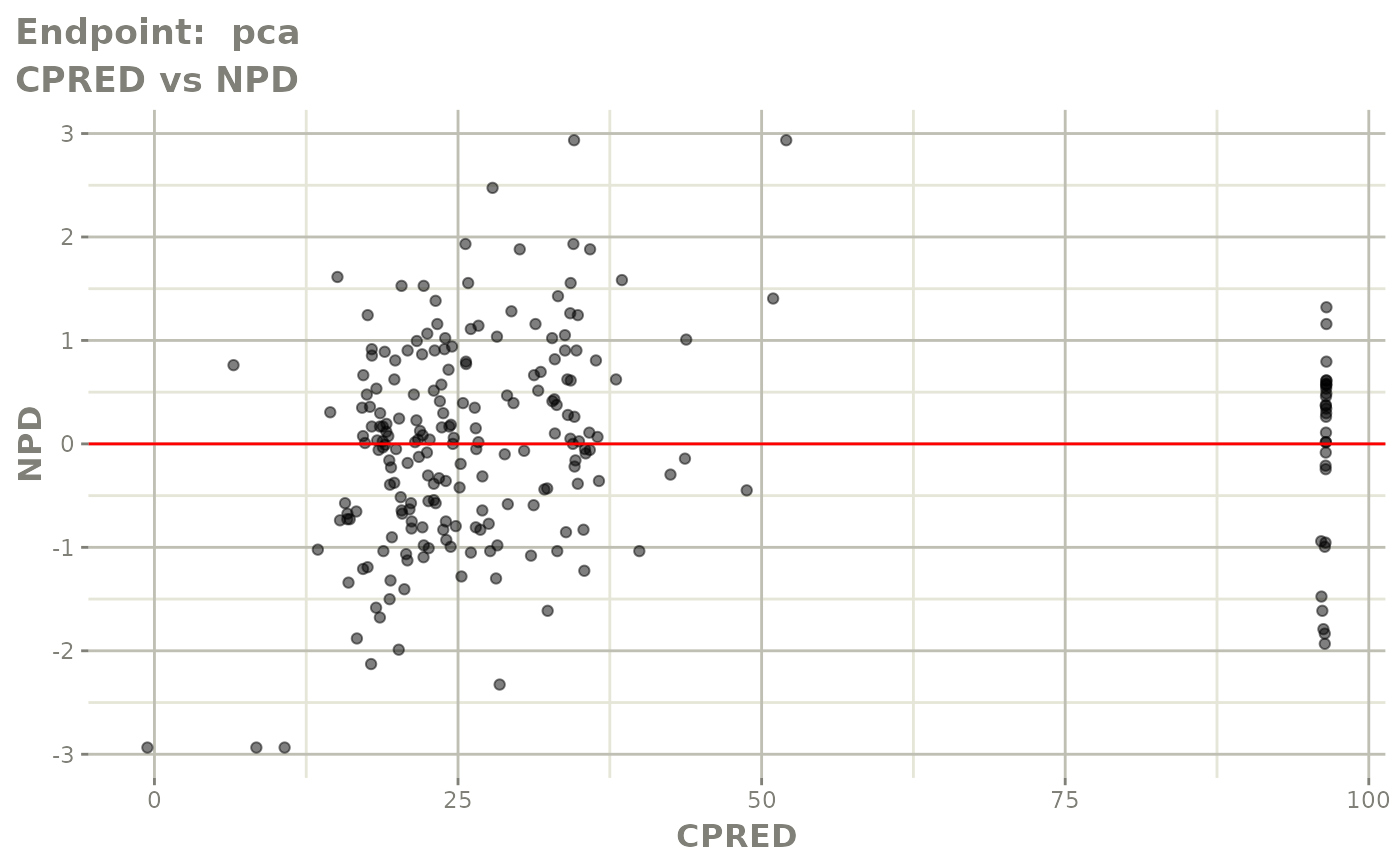
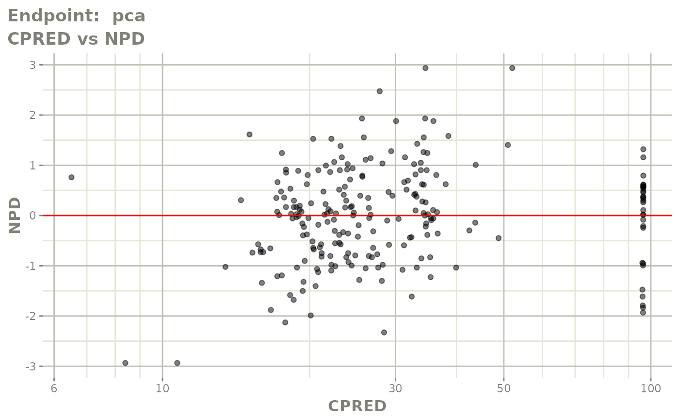
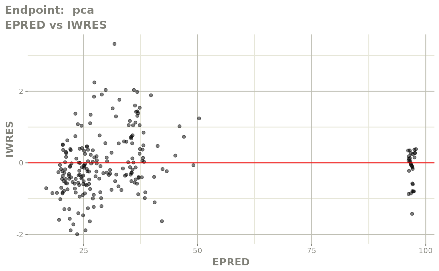
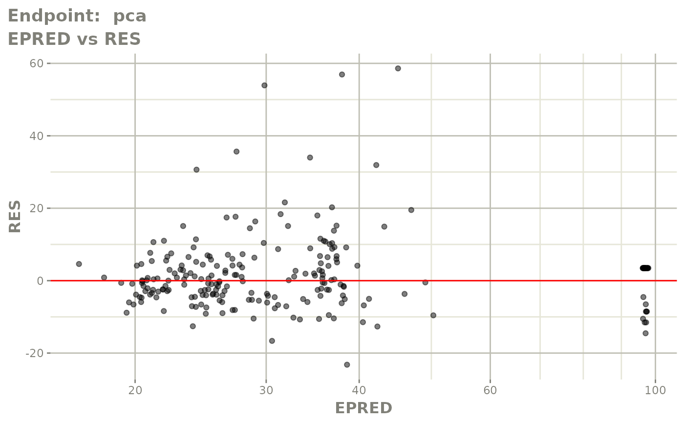
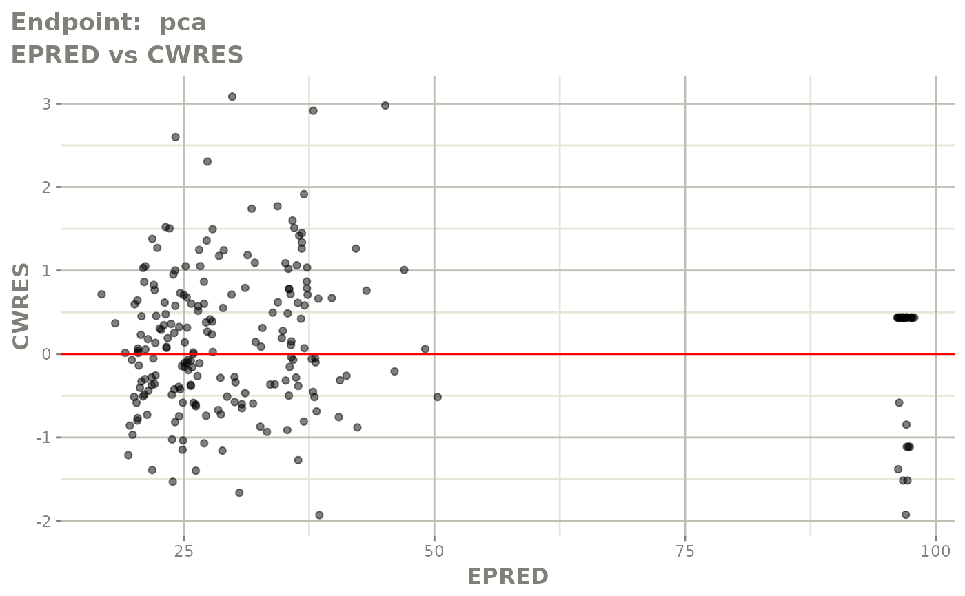
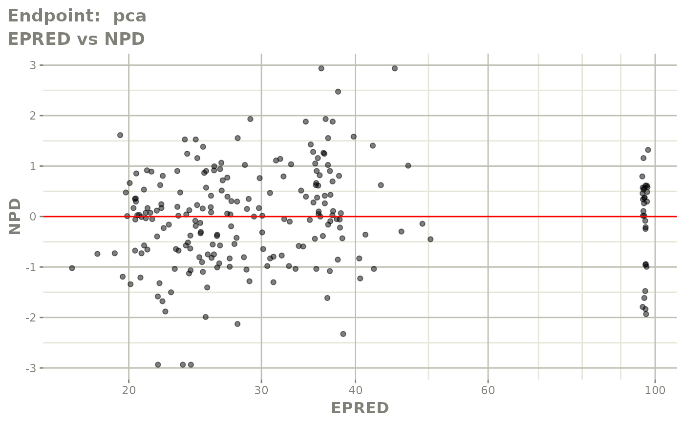
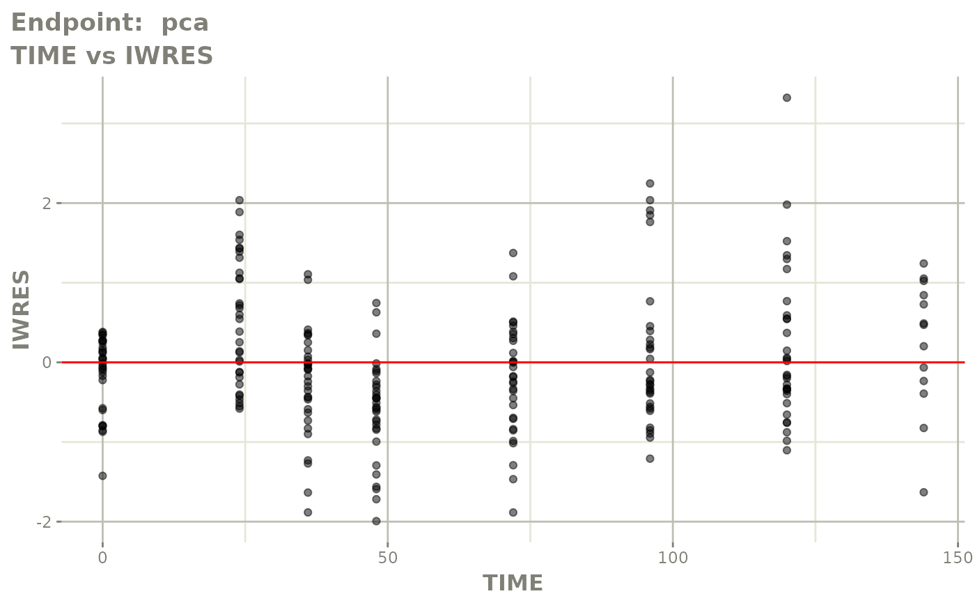
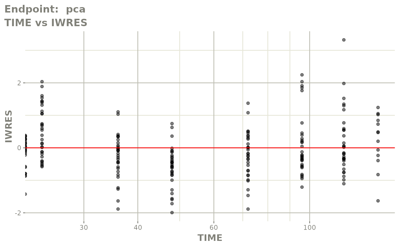
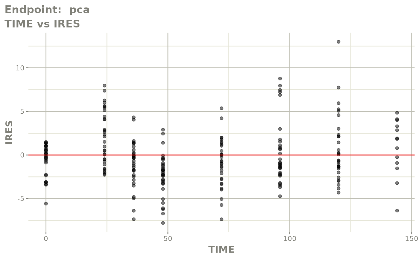
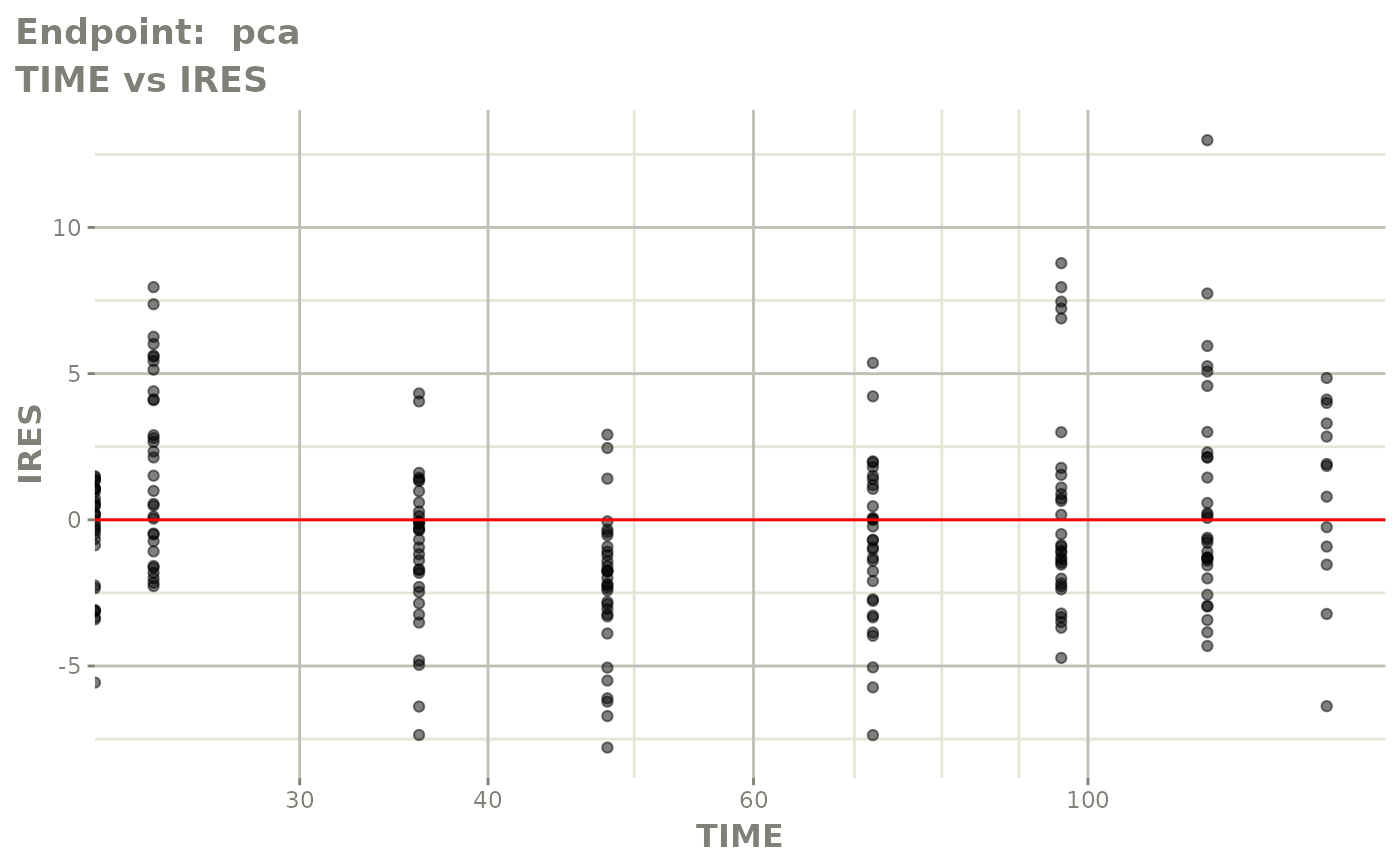
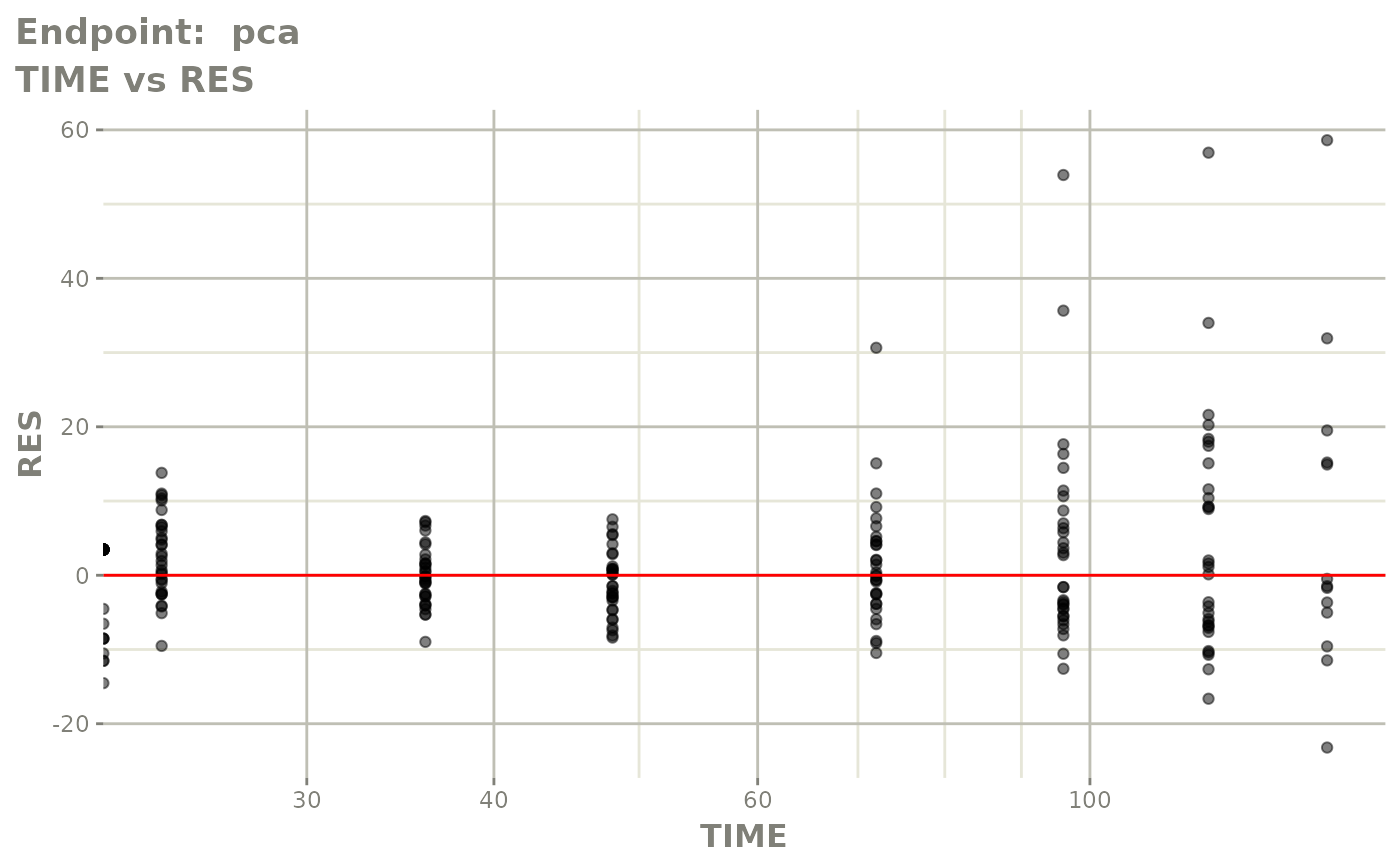
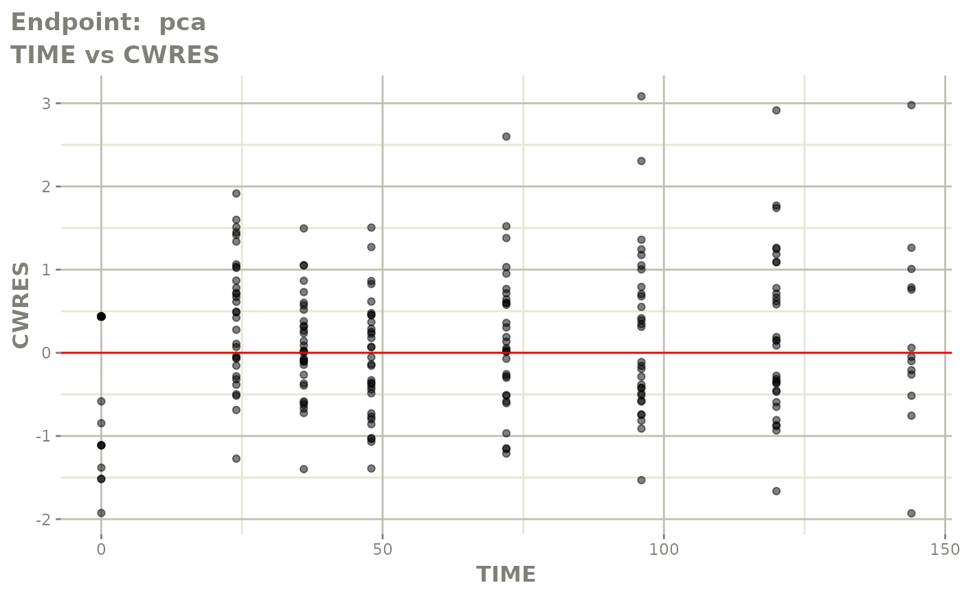
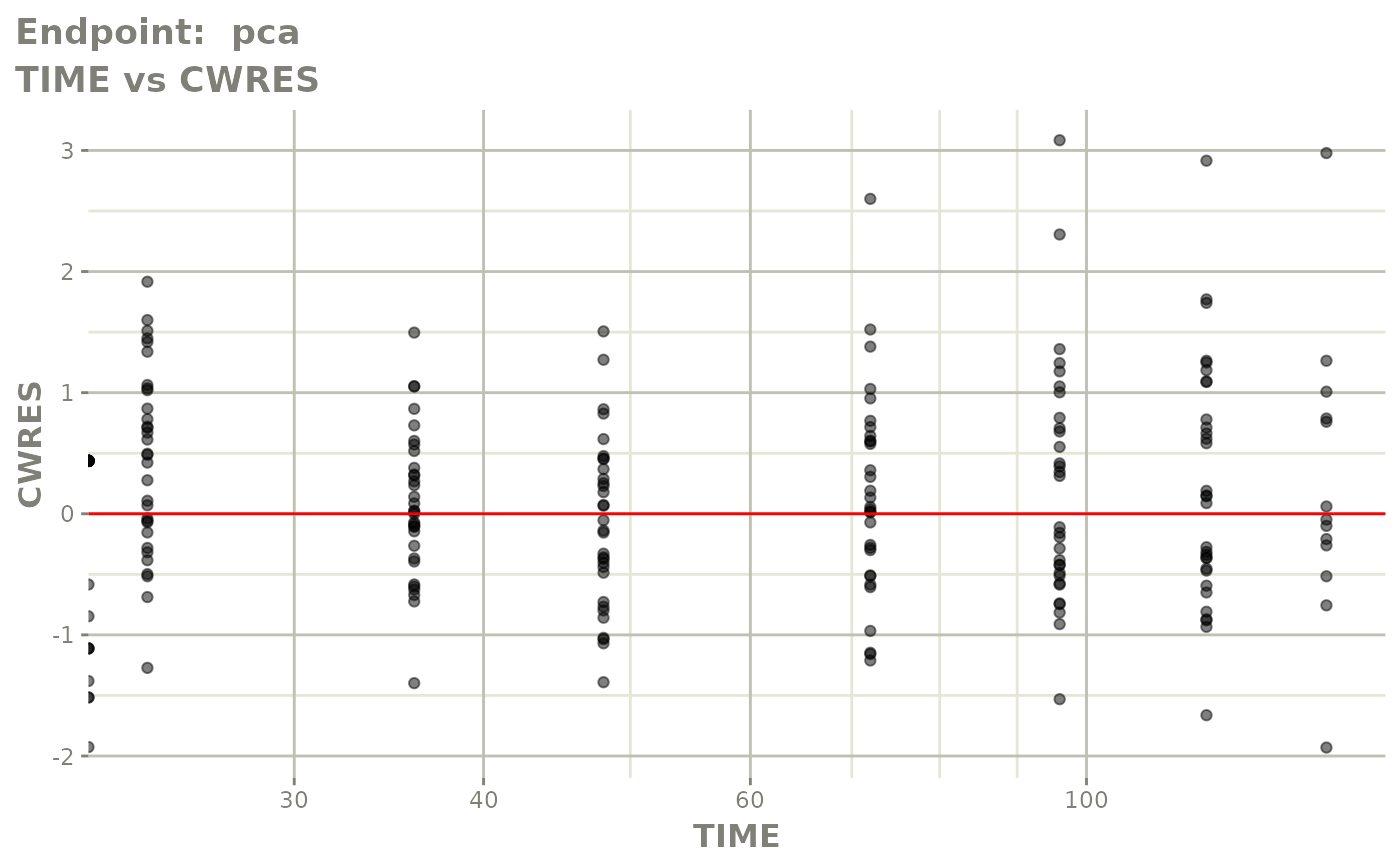
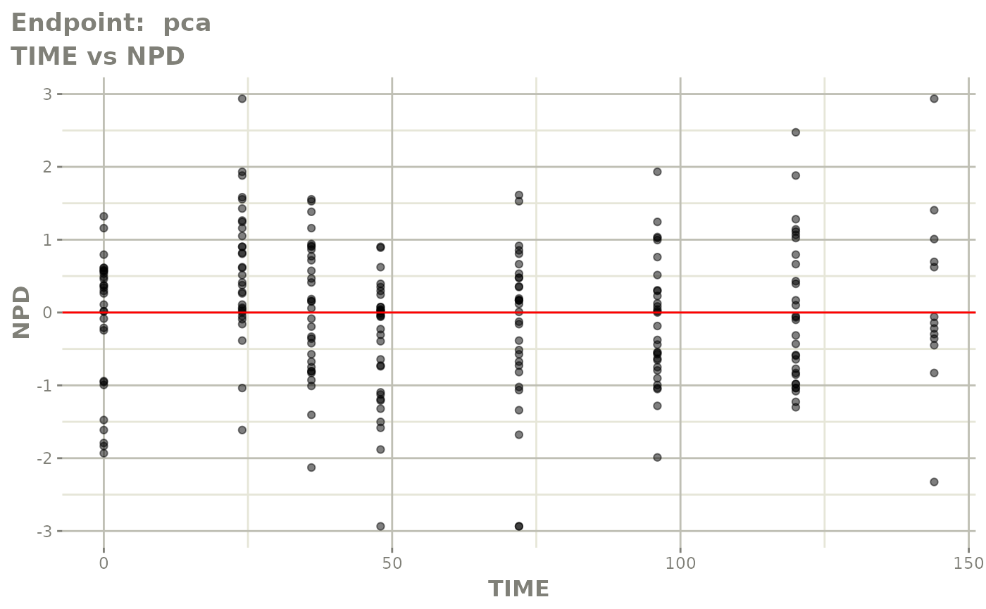
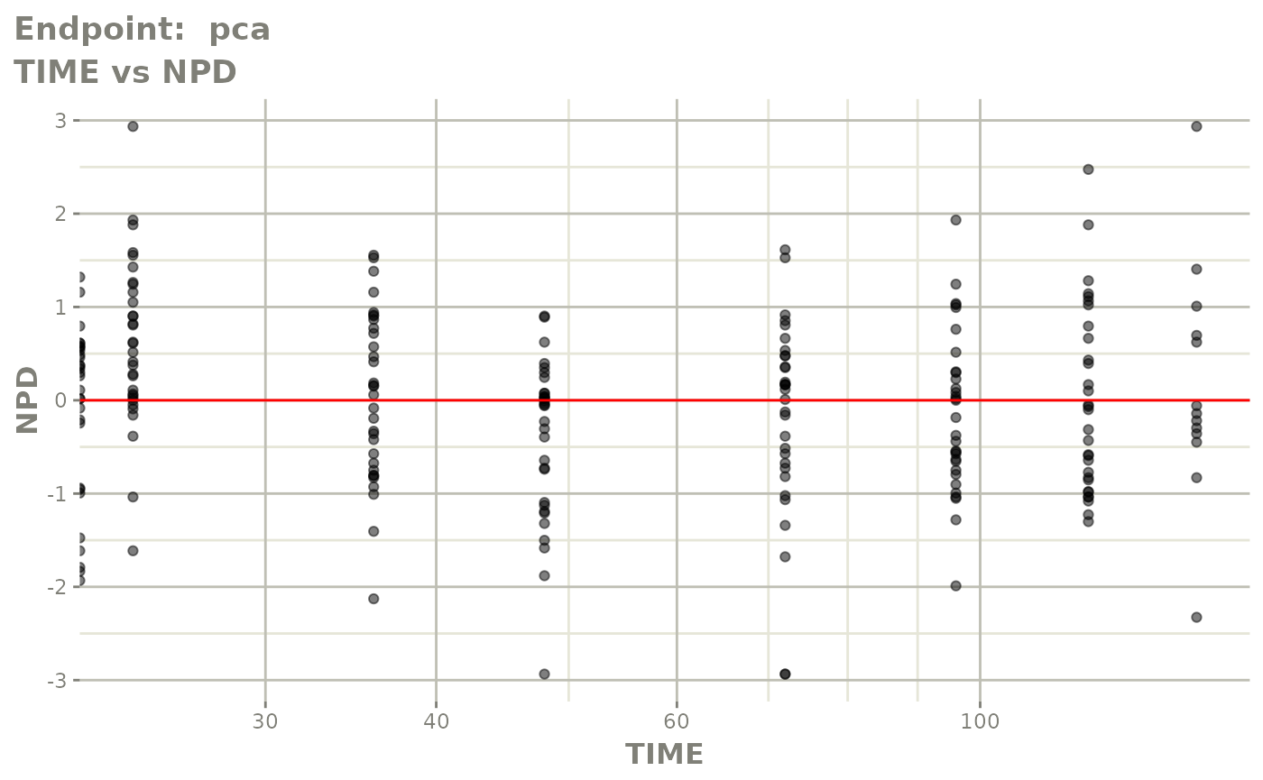
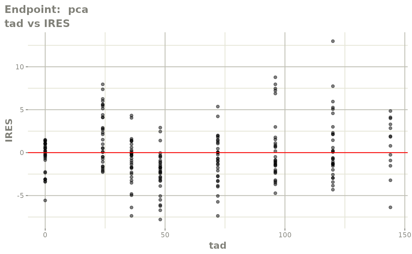
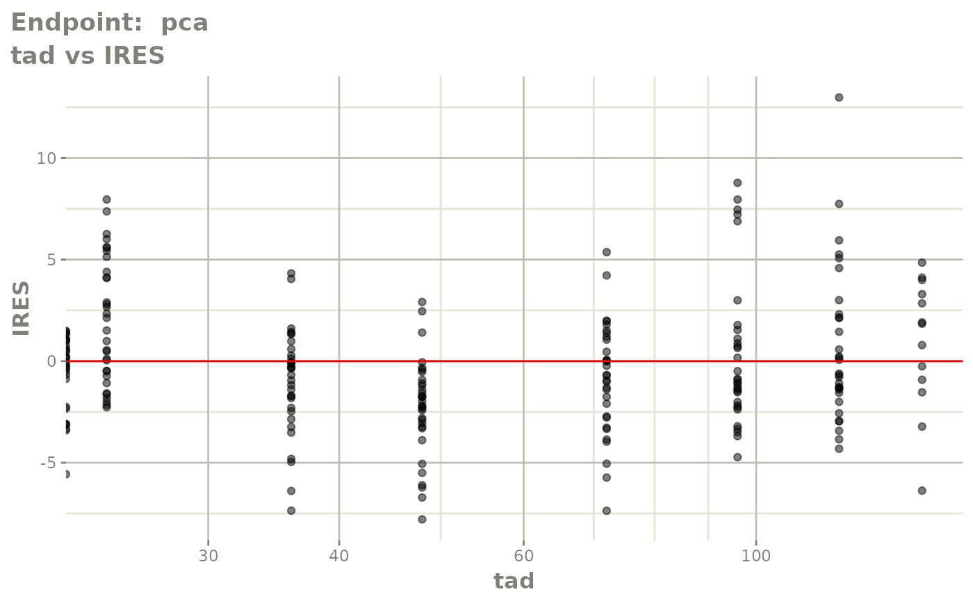
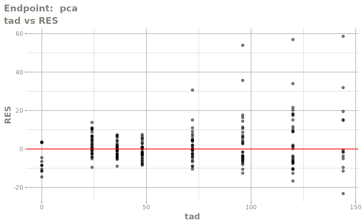
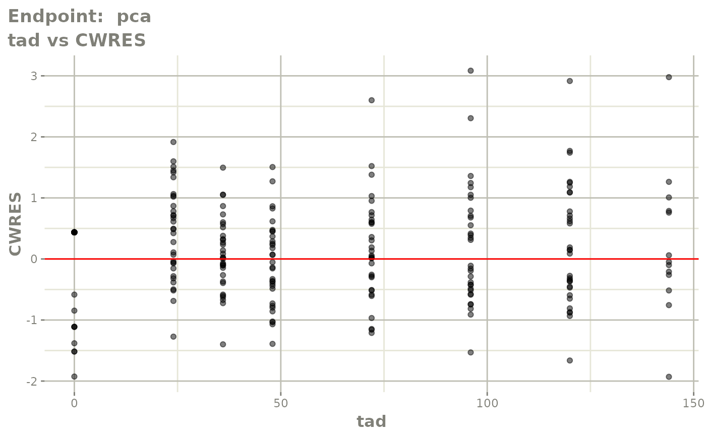
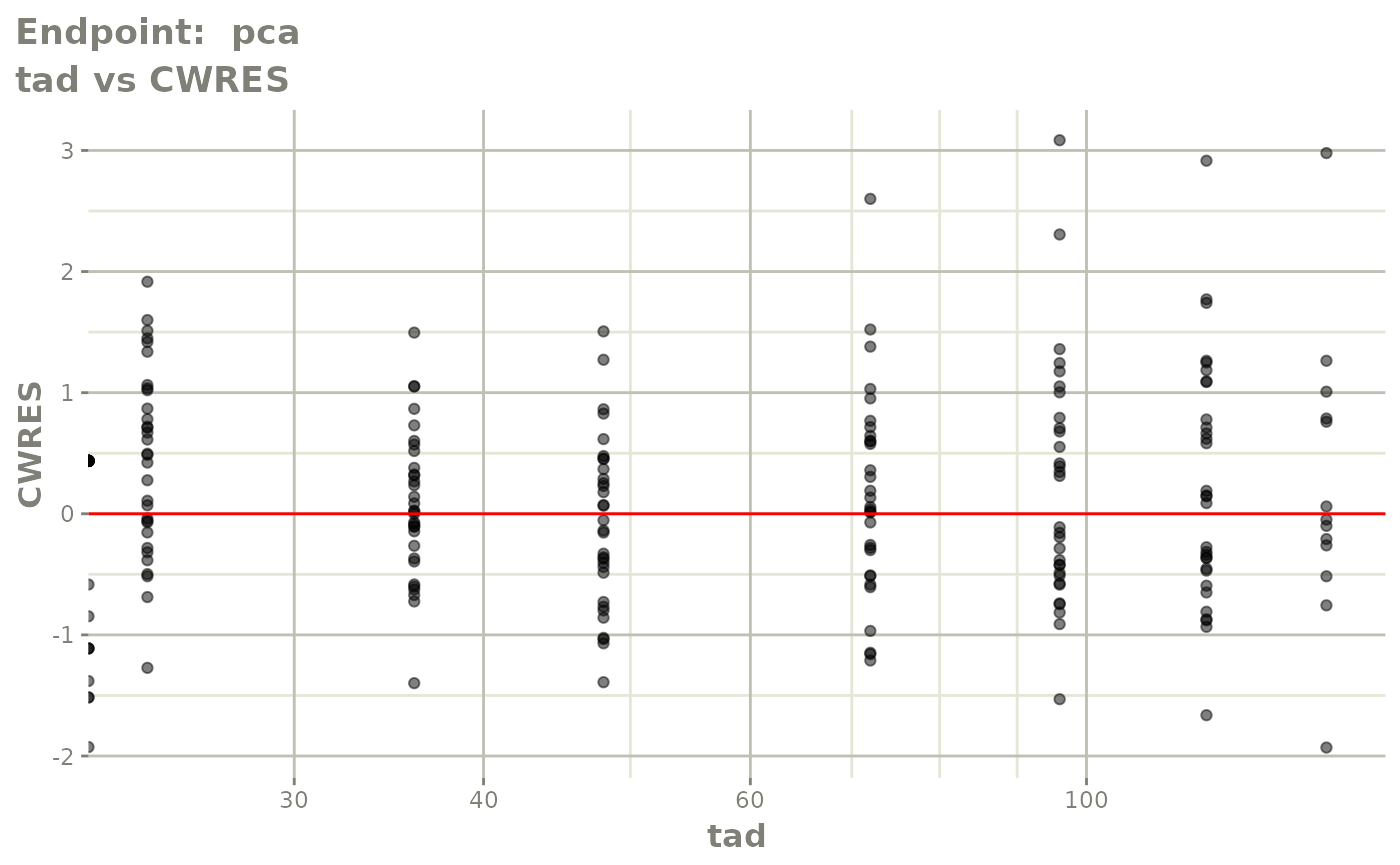
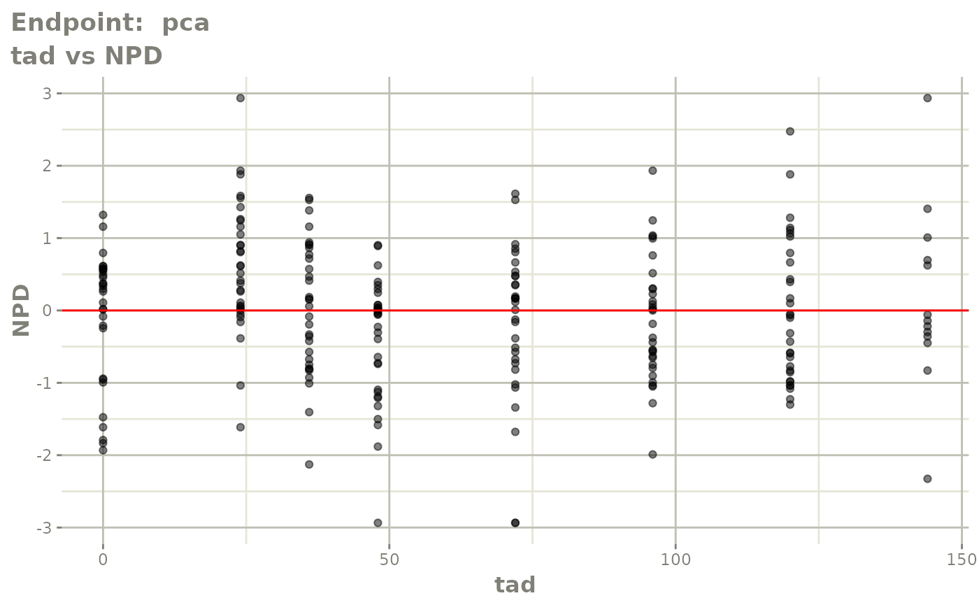
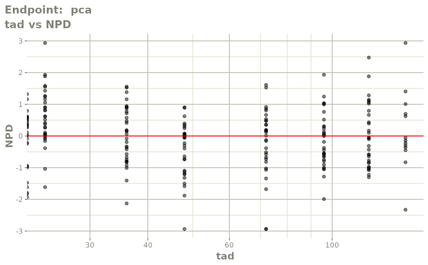
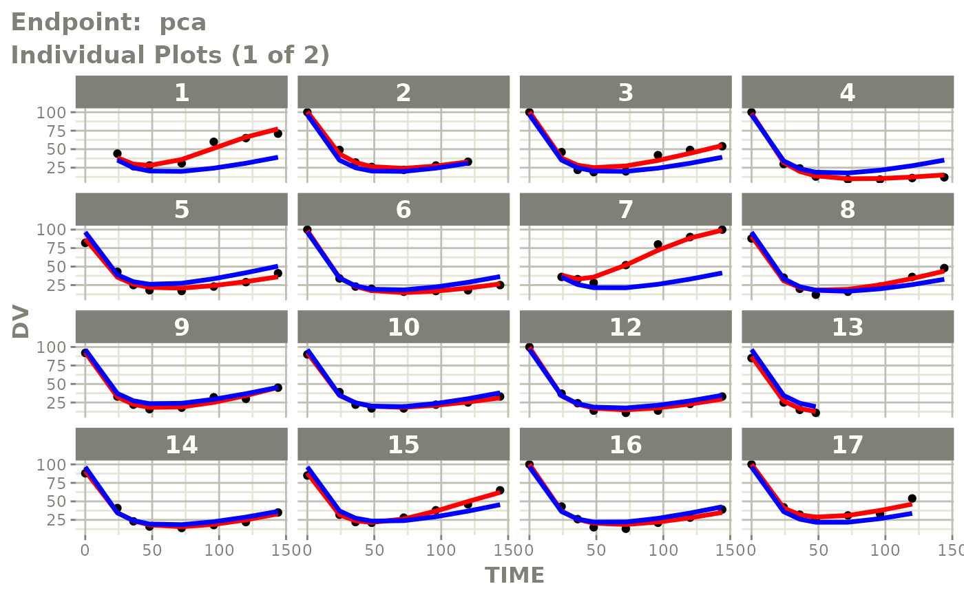
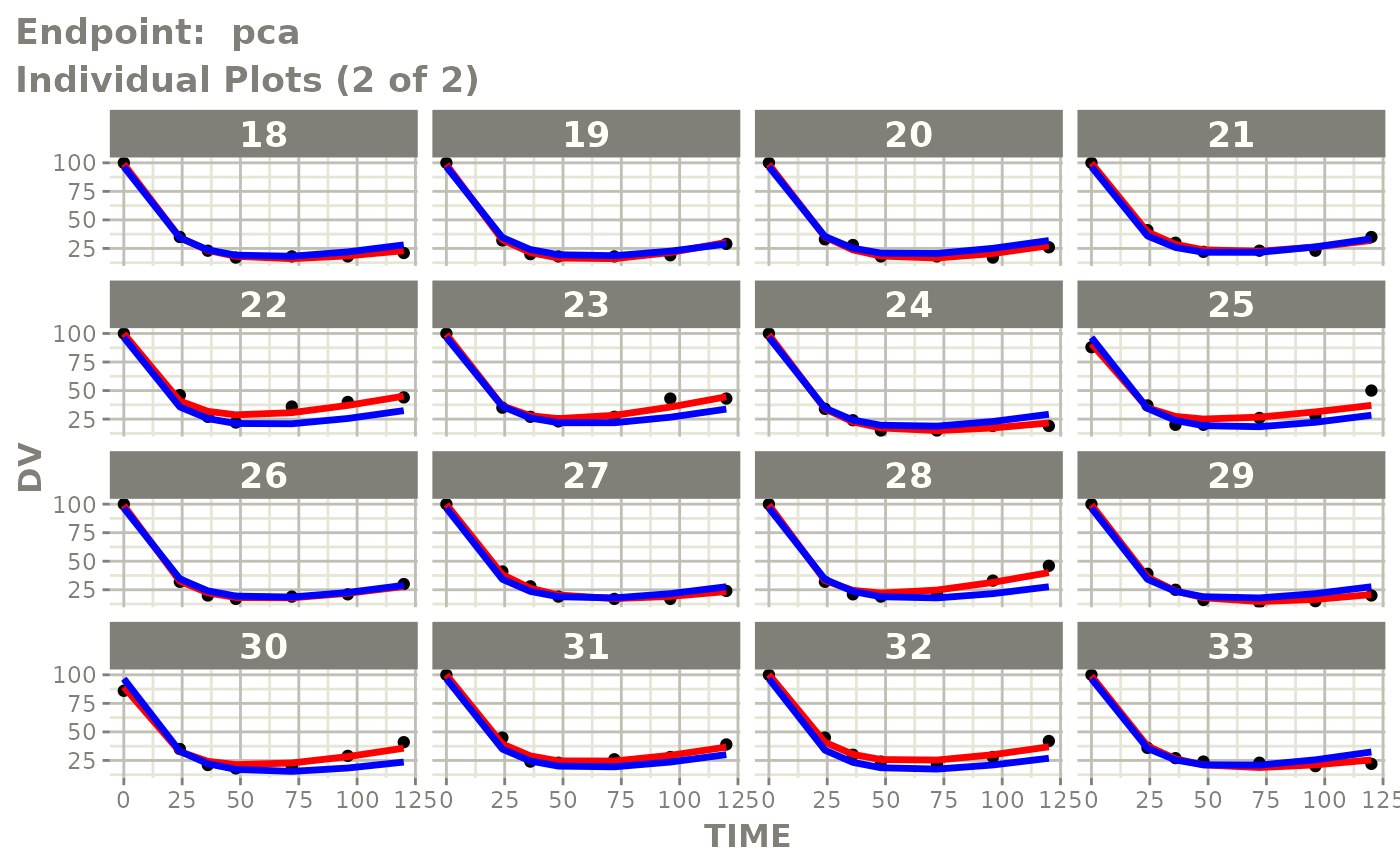
#> # e0 <dbl>, DCP <dbl>, PD <dbl>, kin <dbl>, tad <dbl>, dosenum <dbl>SAEM Diagnostic plots
plot(fit.TOS);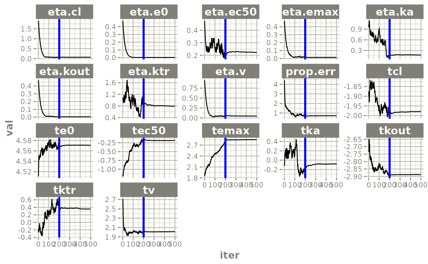


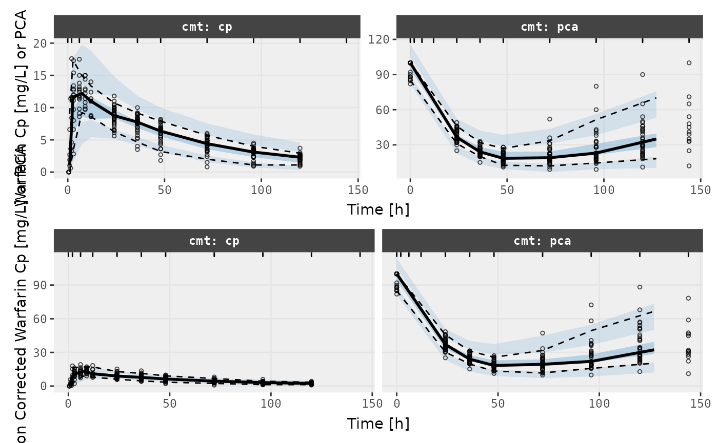
v1s <- nlmixr::vpc(fit.TOS, show=list(obs_dv=T), scales="free_y") +
  ylab("Warfarin Cp [mg/L] or PCA") +
  xlab("Time [h]")

v2s <- nlmixr::vpc(fit.TOS, show=list(obs_dv=T), pred_corr = TRUE) +
  ylab("Prediction Corrected Warfarin Cp [mg/L] or PCA") +
  xlab("Time [h]")

library(patchwork)
v1s / v2s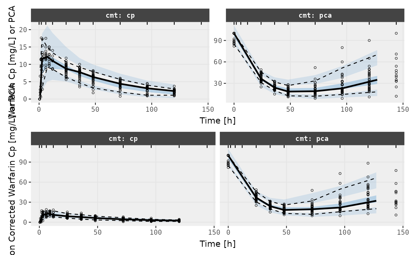
FOCEi fits
## FOCEi fit/vpcs
fit.TOF <- nlmixr(pk.turnover.emax3, warfarin, "focei", control=list(print=0),
table=list(cwres=TRUE, npde=TRUE));
#> [====|====|====|====|====|====|====|====|====|====] 0:00:00
#>
#> [====|====|====|====|====|====|====|====|====|====] 0:00:00
#>
#> [====|====|====|====|====|====|====|====|====|====] 0:00:00
#>
#> [====|====|====|====|====|====|====|====|====|====] 0:00:00
#>
#> [====|====|====|====|====|====|====|====|====|====] 0:00:00
#>
#> [====|====|====|====|====|====|====|====|====|====] 0:00:00
#>
#> [====|====|====|====|====|====|====|====|====|====] 0:00:00
#>
#> [====|====|====|====|====|====|====|====|====|====] 0:00:00
#>
#> [====|====|====|====|====|====|====|====|====|====] 0:00:00
#>
#> [====|====|====|====|====|====|====|====|====|====] 0:00:00
#>
#> [1] "CMT"
#> calculating covariance matrix
#> [====|====|====|====|====|====|====|====|====|====] 0:01:17
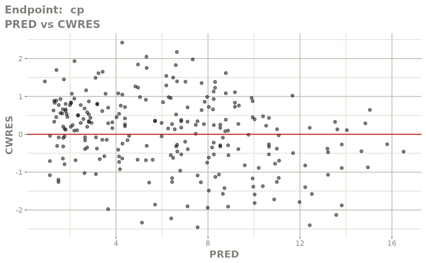
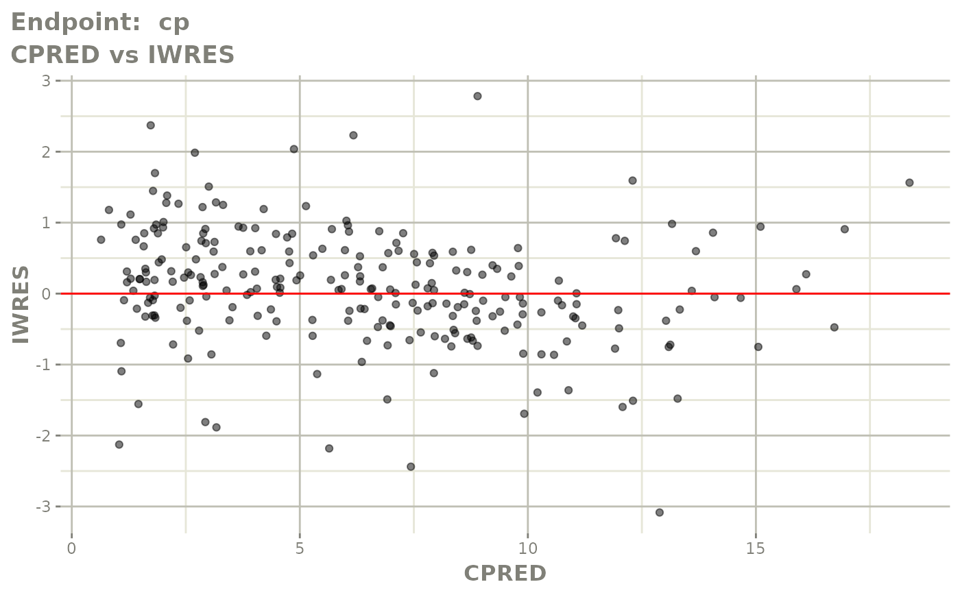
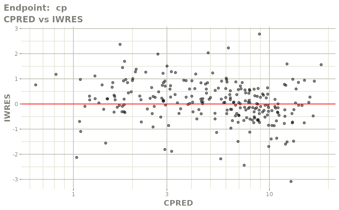
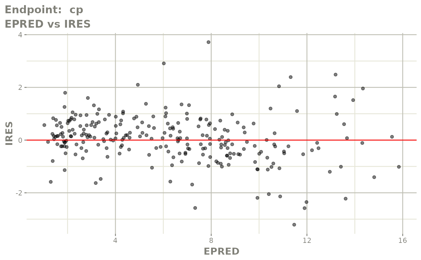
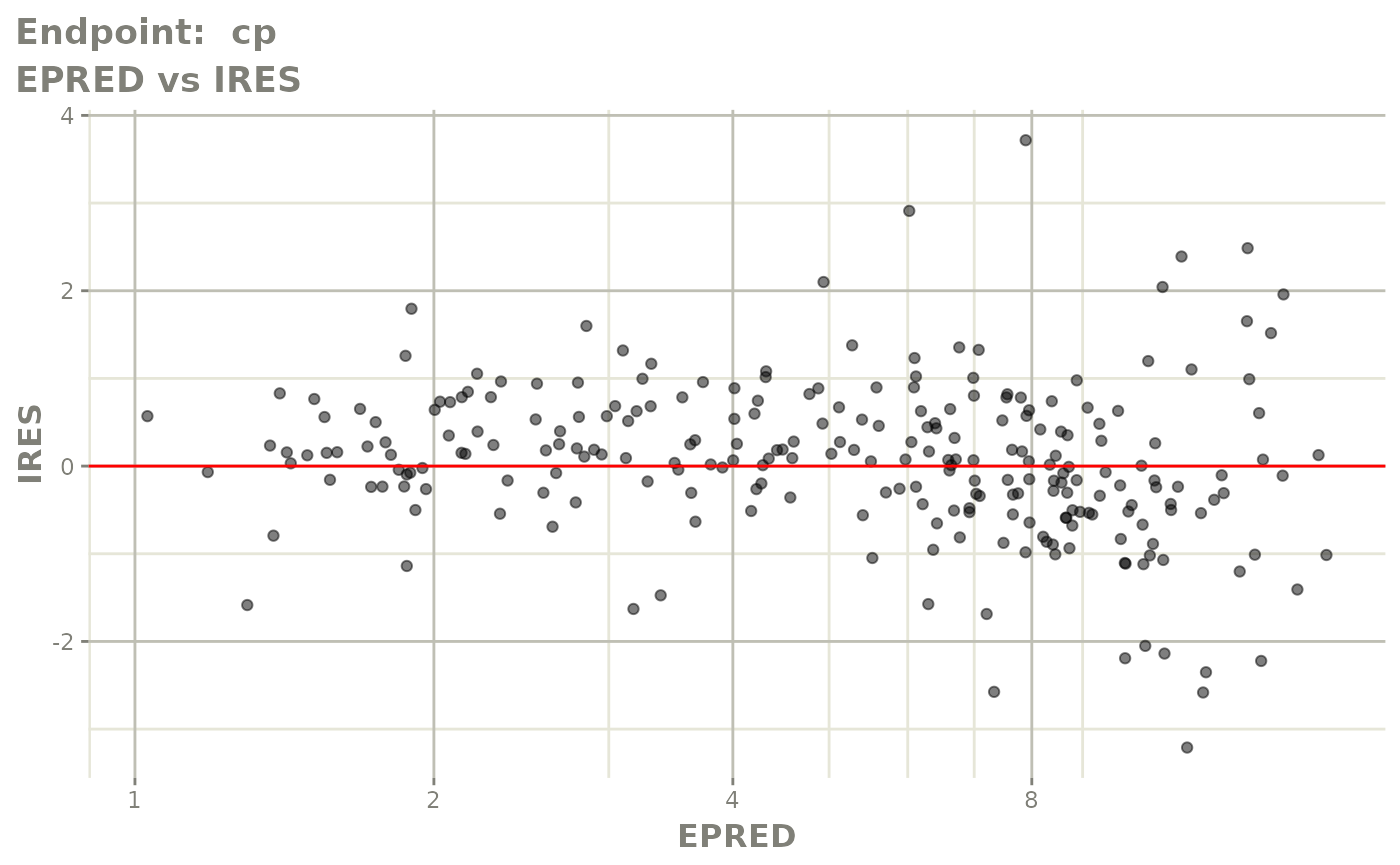
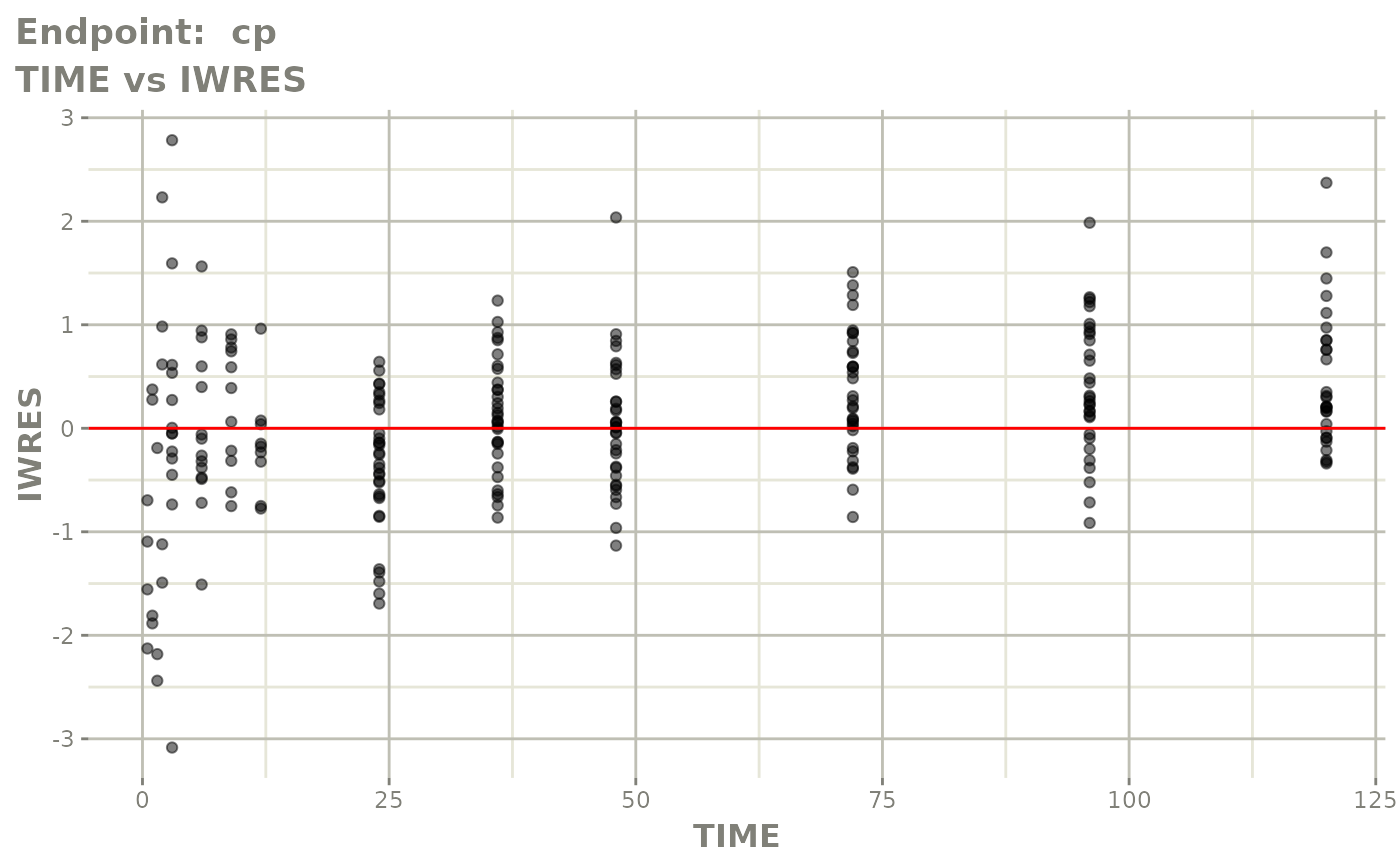
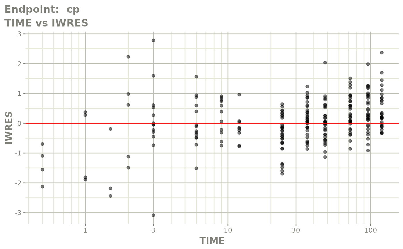
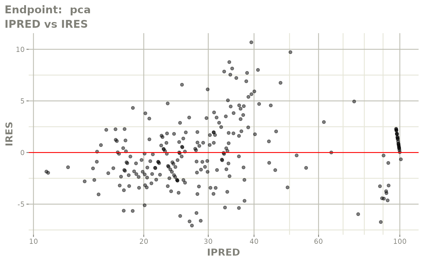
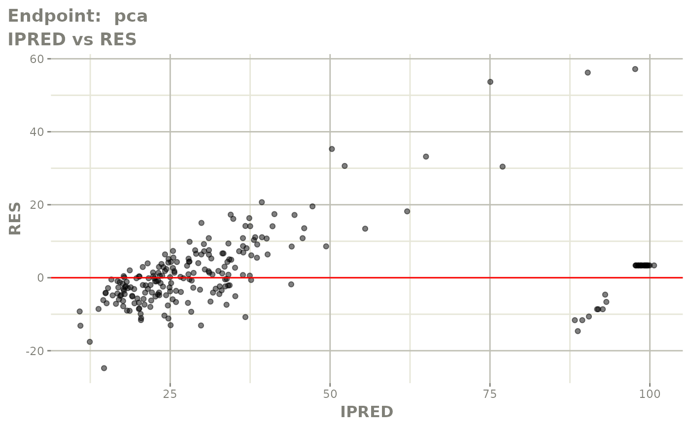
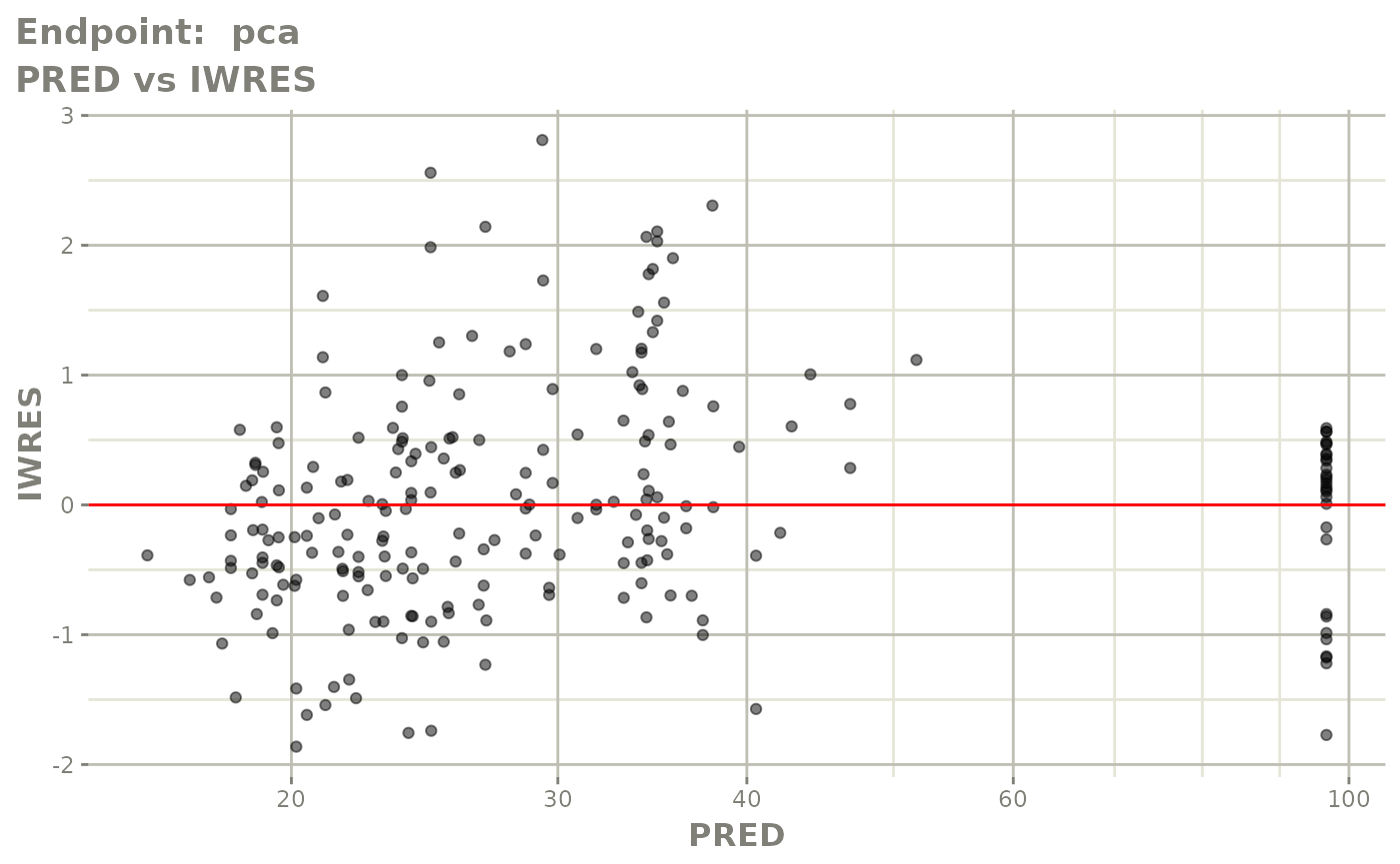
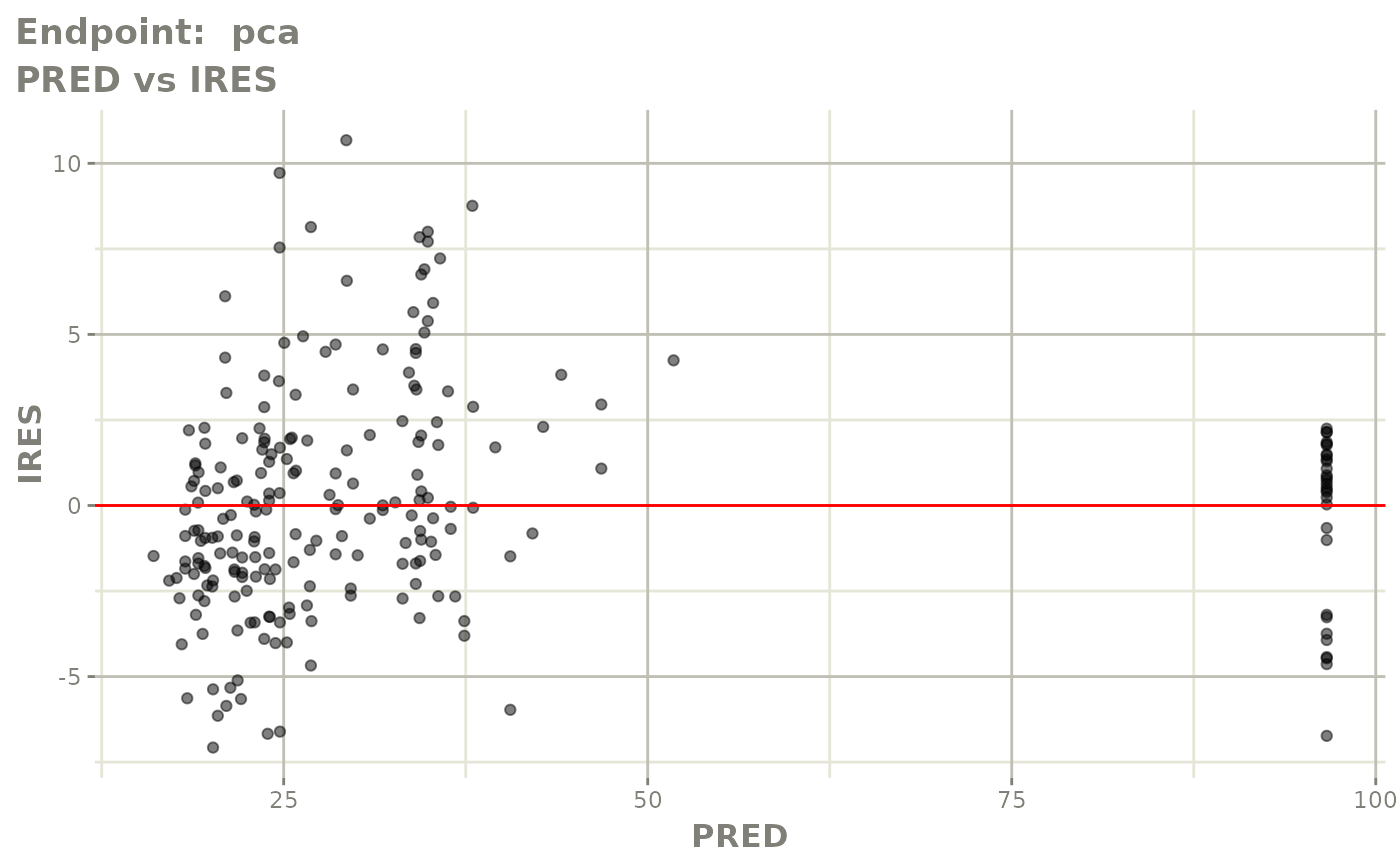
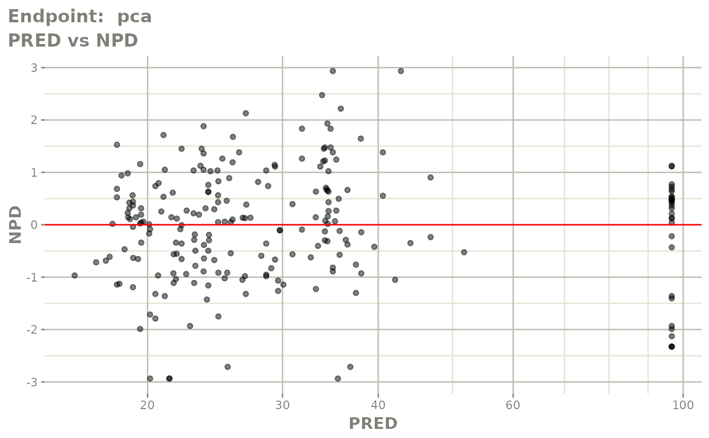
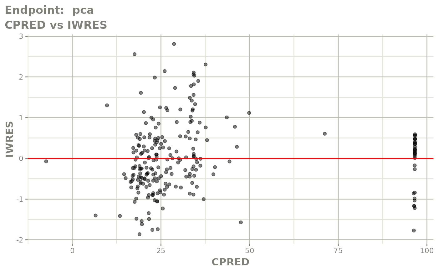
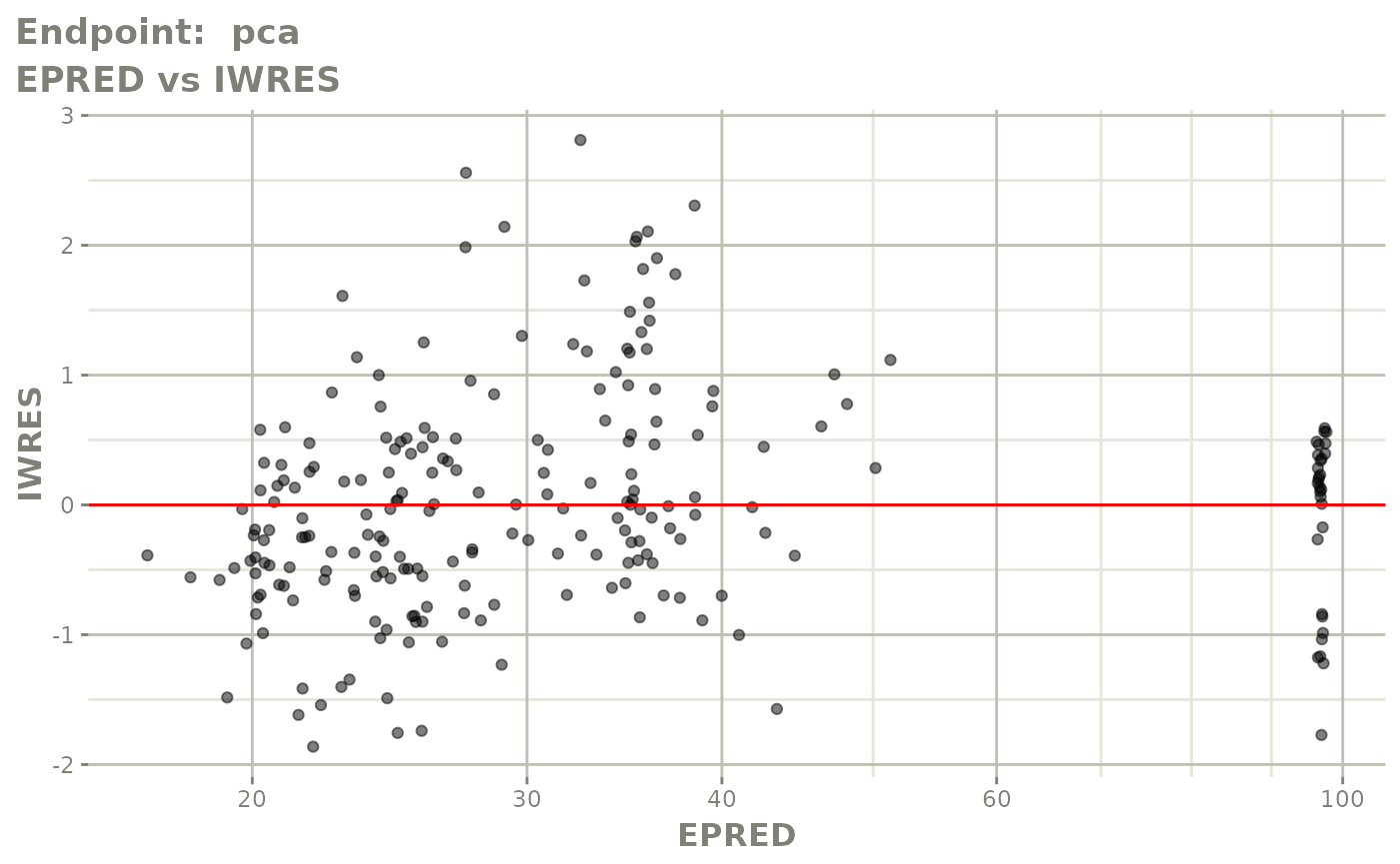
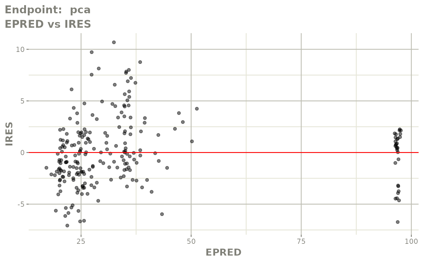
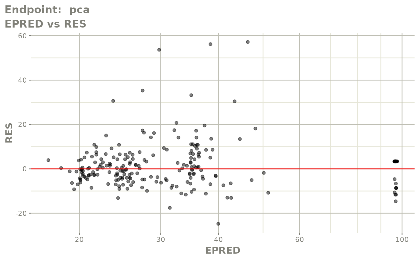
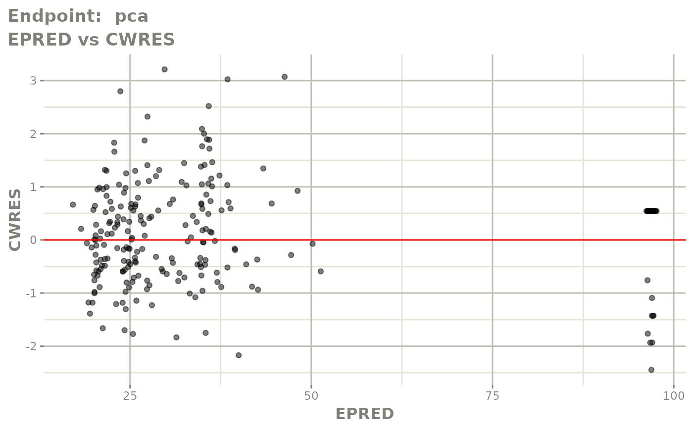
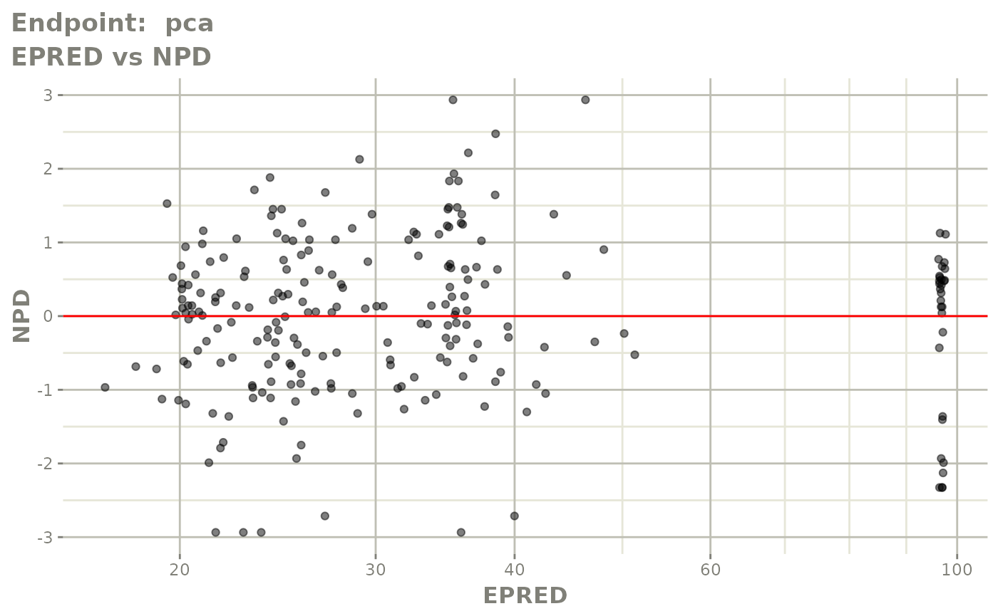
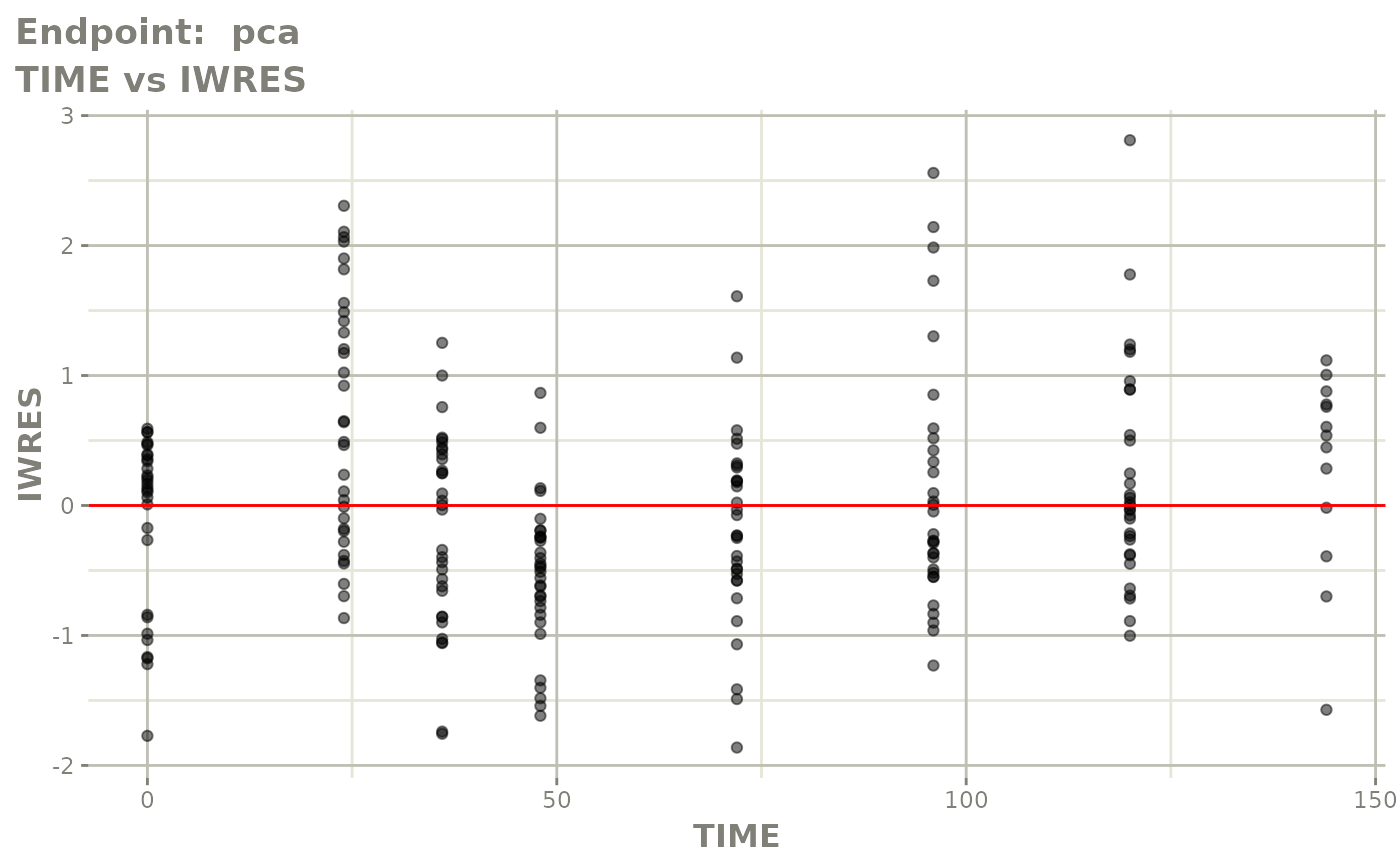
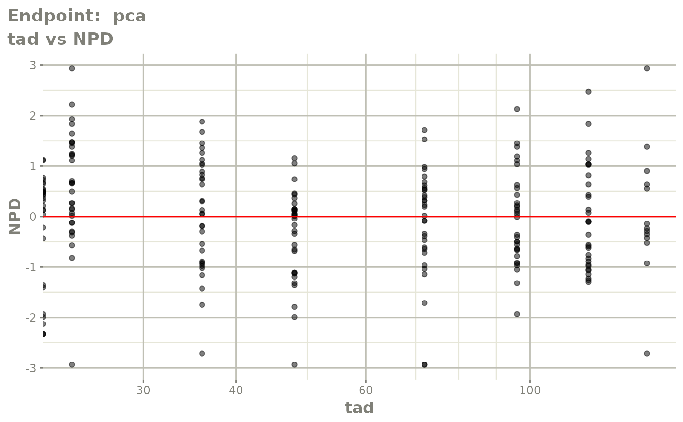
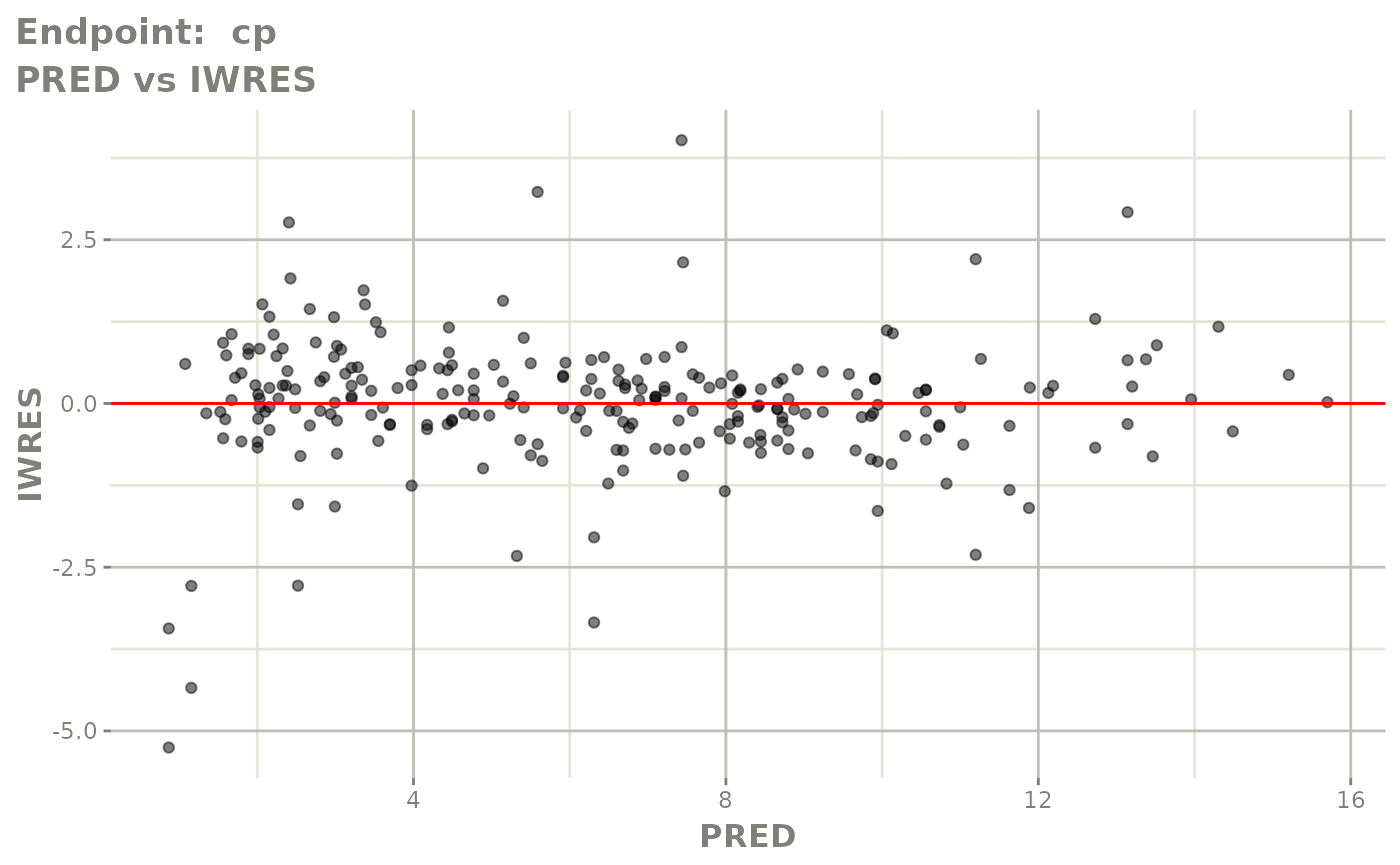
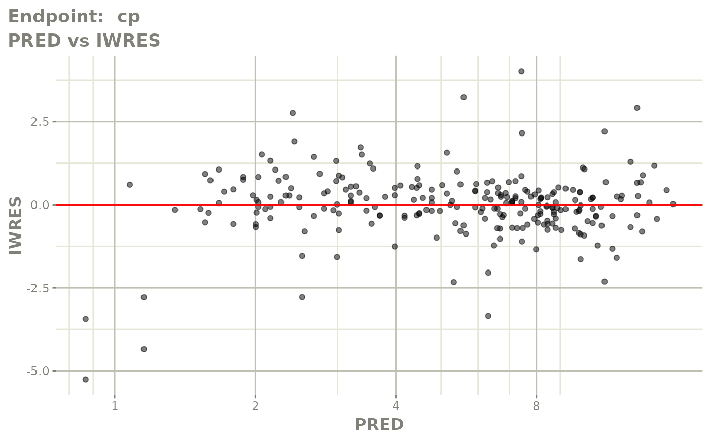
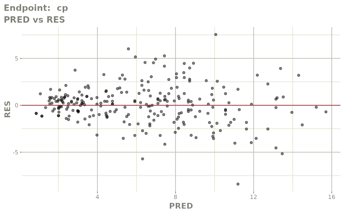
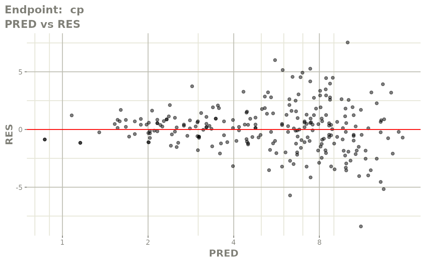
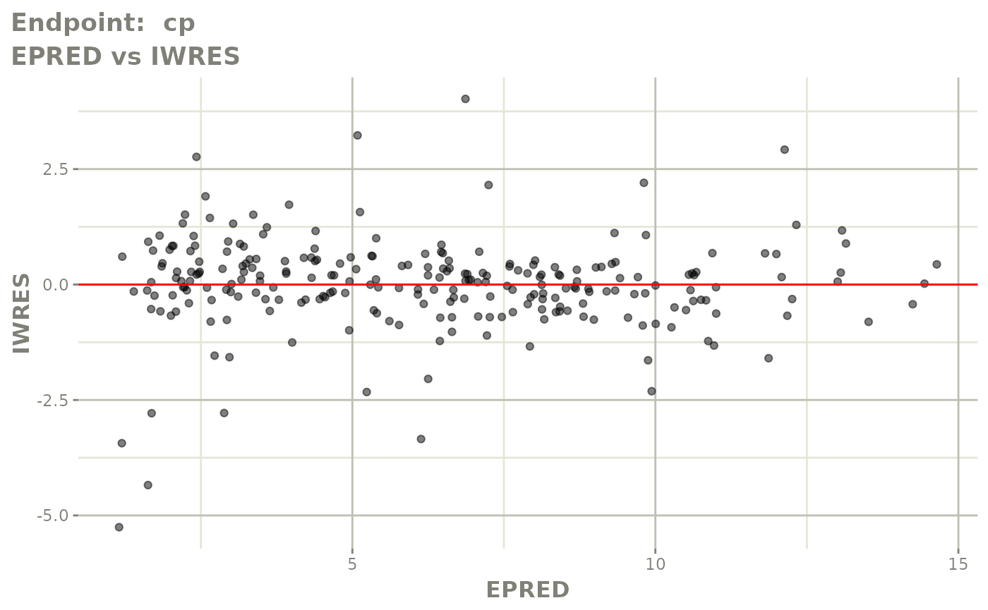
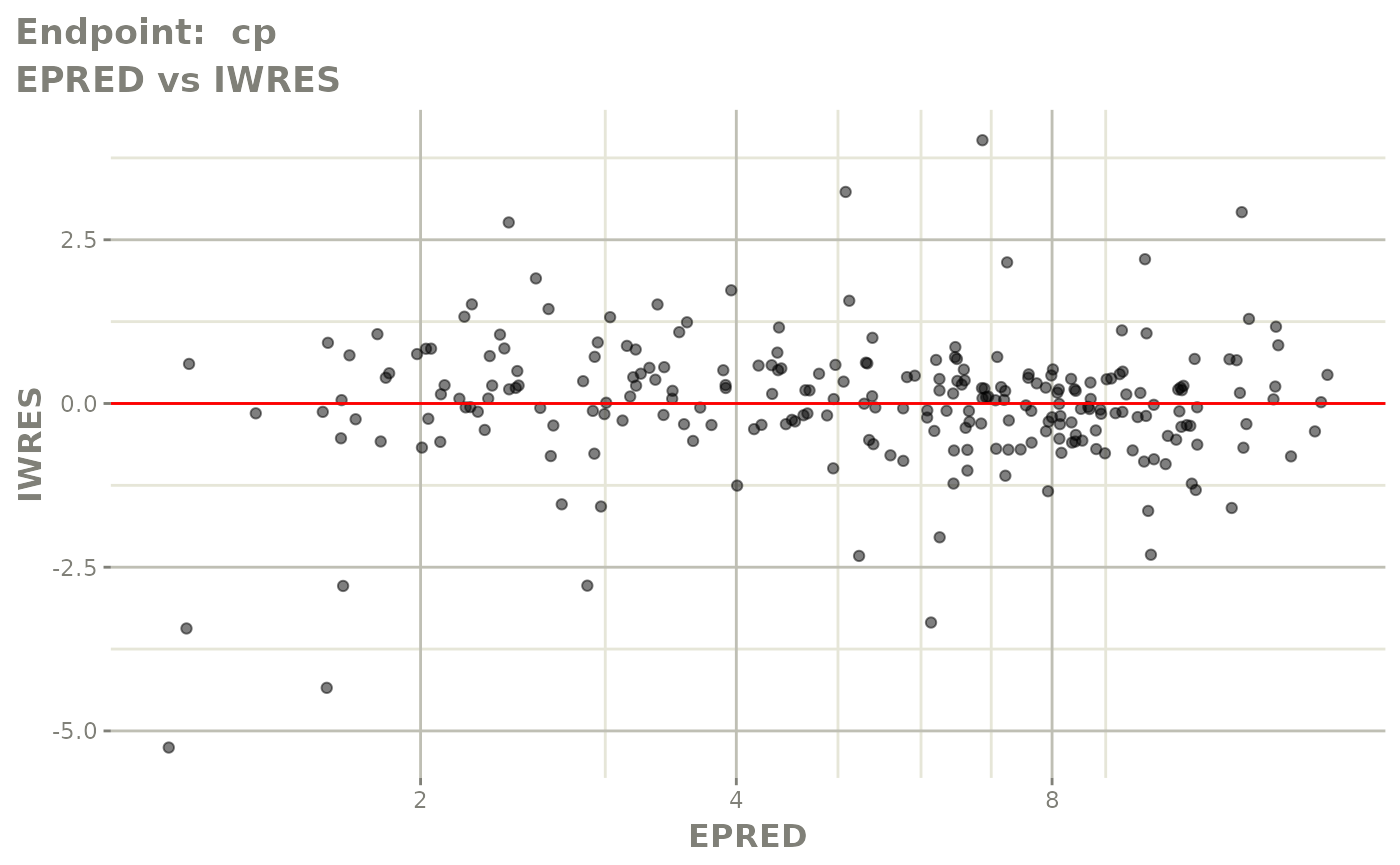
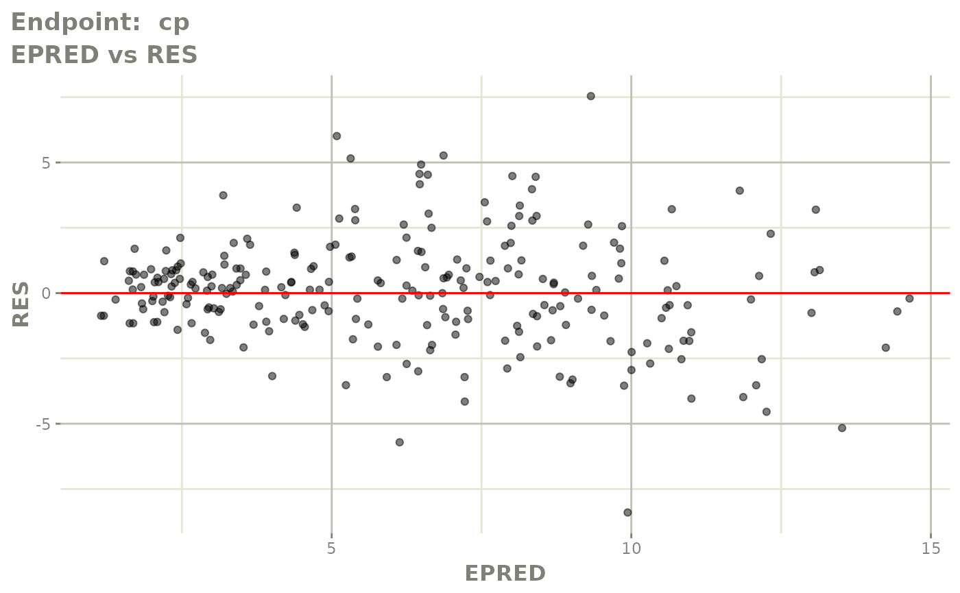
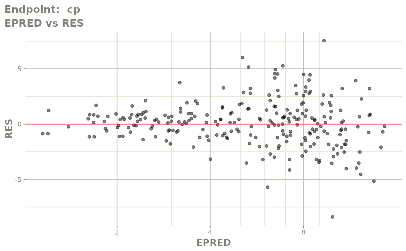
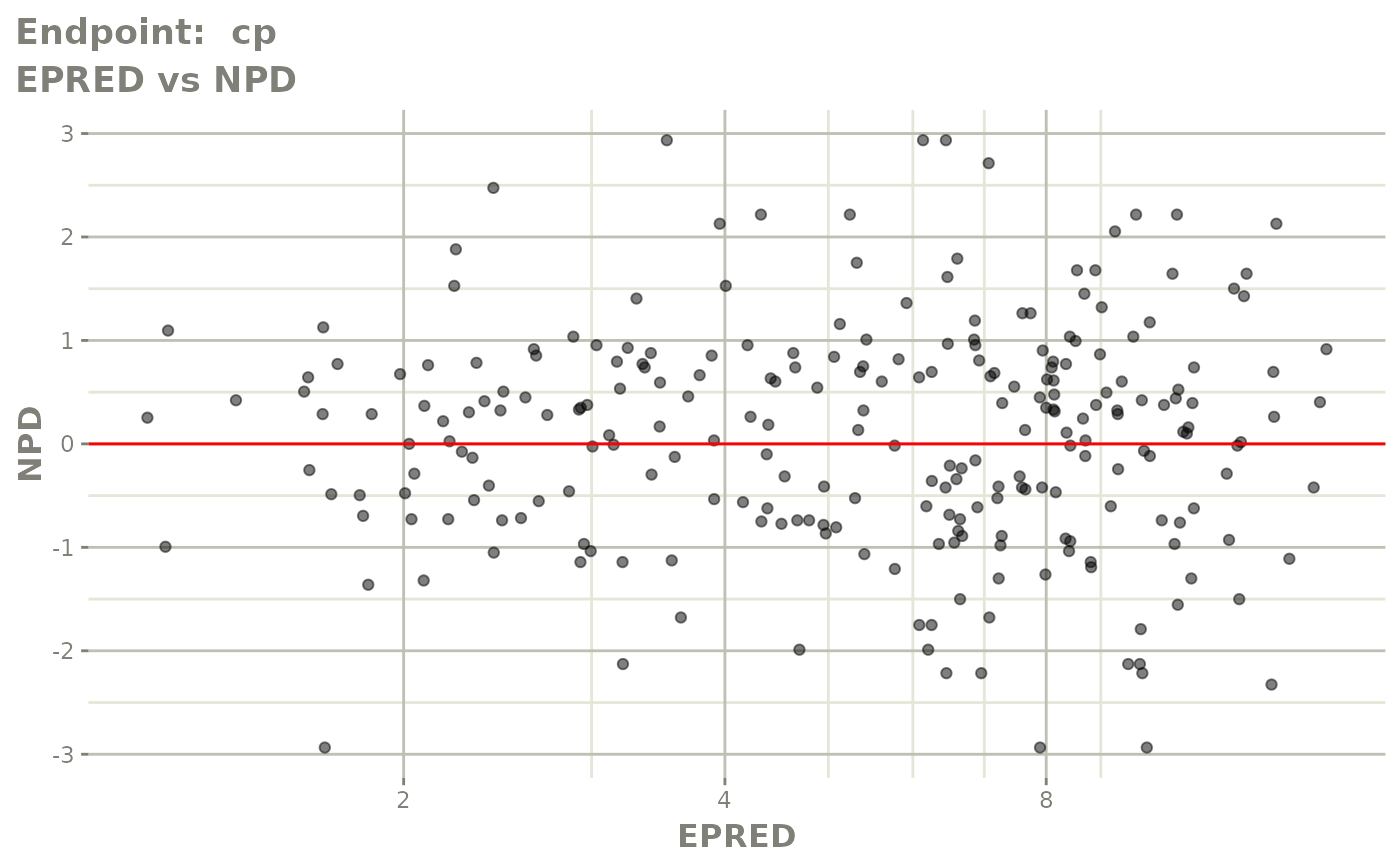
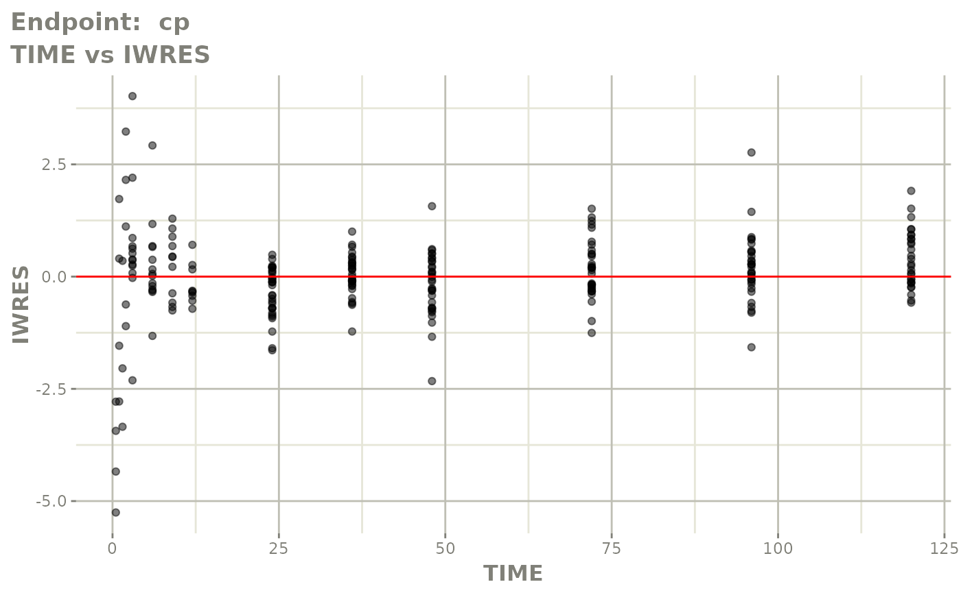
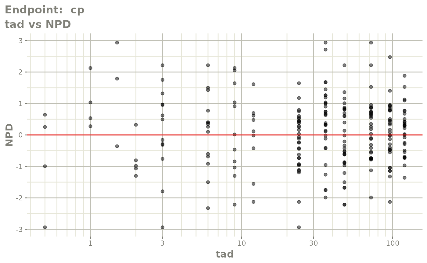
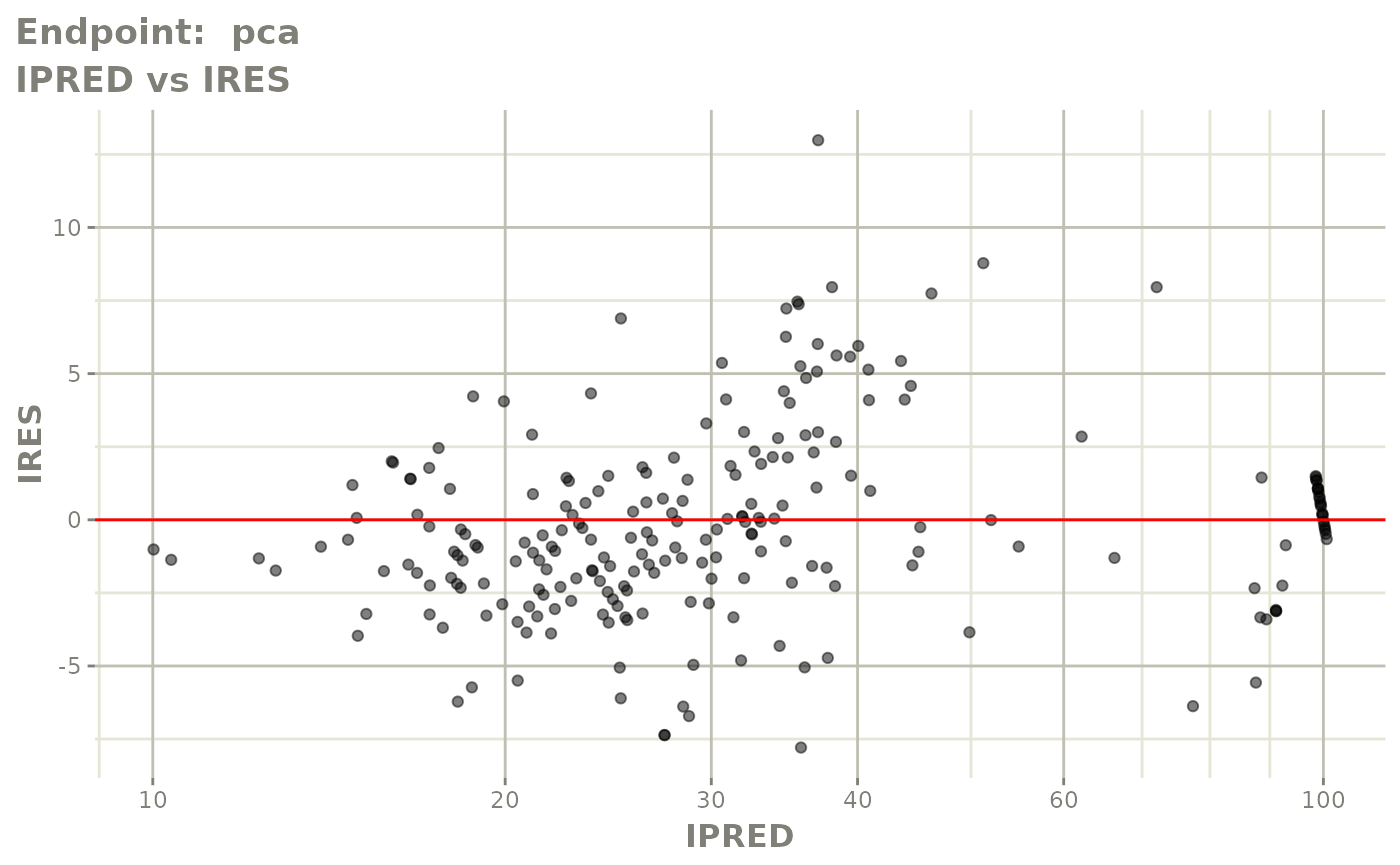
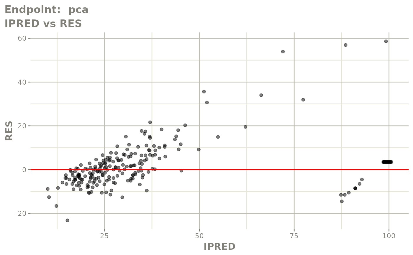
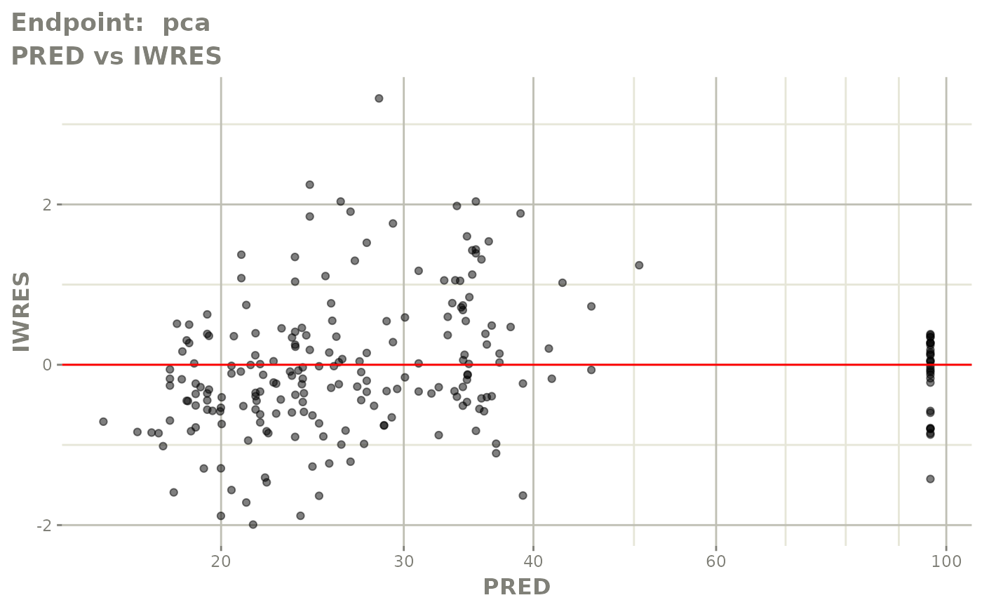
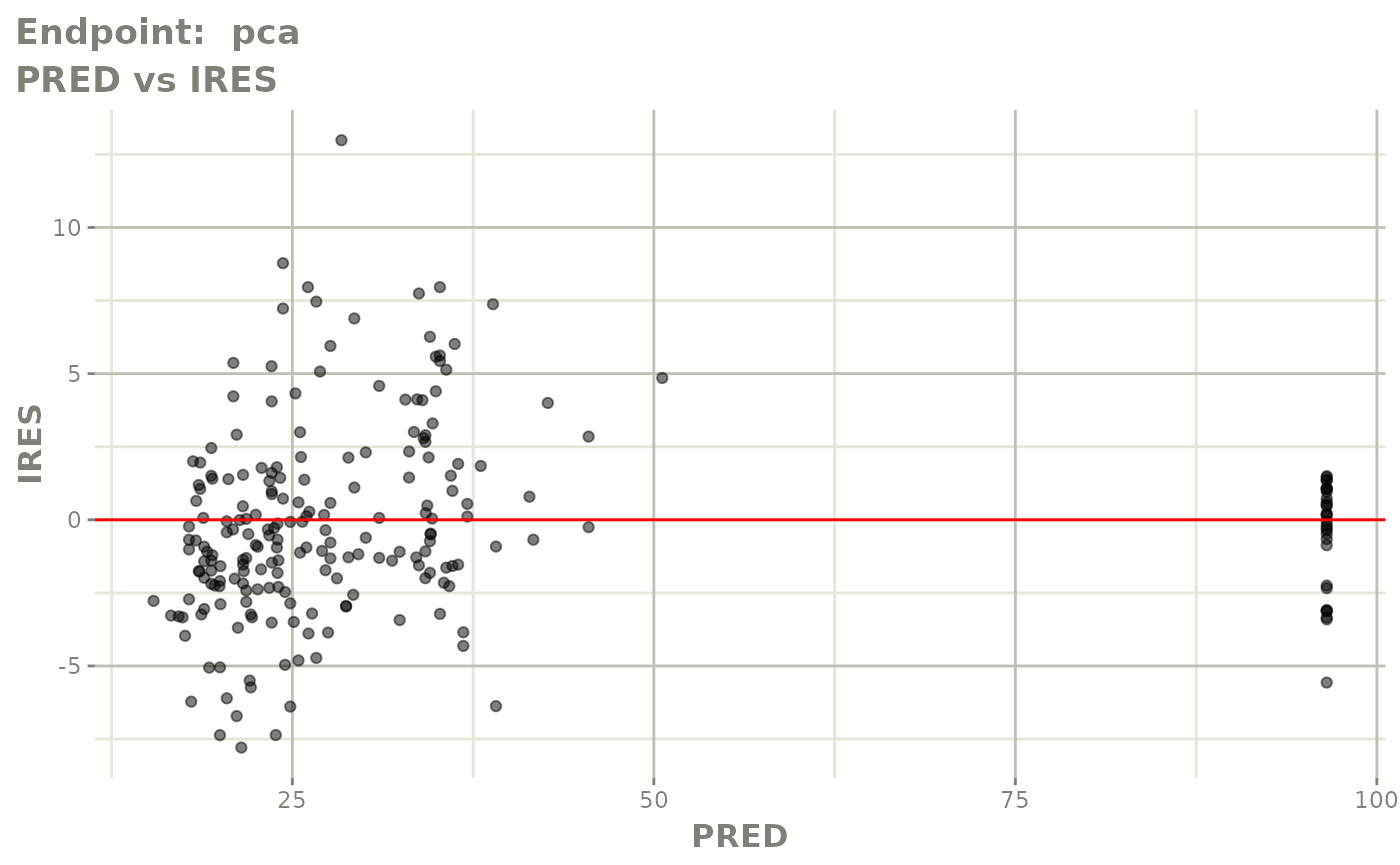
#> doneFOCEi Diagnostic Plots
print(fit.TOF)
#> ── nlmixr FOCEi (outer: nlminb) fit ────────────────────────────────────────────
#>
#> OBJF AIC BIC Log-likelihood Condition Number
#> FOCEi 1421.704 2347.399 2426.819 -1154.7 1380.116
#>
#> ── Time (sec $time): ───────────────────────────────────────────────────────────
#>
#> setup optimize covariance table other
#> elapsed 19.61535 77.61424 77.61425 2.754 72.26916
#>
#> ── Population Parameters ($parFixed or $parFixedDf): ───────────────────────────
#>
#> Est. SE %RSE Back-transformed(95%CI) BSV(CV% or SD)
#> tktr 0.106 0.0895 84.7 1.11 (0.933, 1.32) 105.
#> tka -0.087 0.138 159 0.917 (0.699, 1.2) 90.6
#> tcl -2.03 0.0309 1.52 0.131 (0.123, 0.139) 28.1
#> tv 2.07 0.0945 4.57 7.9 (6.56, 9.5) 22.9
#> prop.err 0.15 0.15
#> pkadd.err 0.144 0.144
#> temax 3.4 0.19 5.6 0.968 (0.954, 0.977) 0.509
#> tec50 0.00724 0.0837 1.16e+03 1.01 (0.855, 1.19) 51.9
#> tkout -2.9 0.0285 0.981 0.0548 (0.0518, 0.0579) 12.7
#> te0 4.57 0.00636 0.139 96.5 (95.3, 97.7) 7.08
#> pdadd.err 3.91 3.91
#> Shrink(SD)%
#> tktr 60.0%
#> tka 60.8%
#> tcl 2.85%
#> tv 11.0%
#> prop.err
#> pkadd.err
#> temax 84.1%
#> tec50 6.49%
#> tkout 30.5%
#> te0 24.5%
#> pdadd.err
#>
#> Covariance Type ($covMethod): r,s
#> Some strong fixed parameter correlations exist ($cor) :
#> cor:tka,tktr cor:tcl,tktr cor:tv,tktr cor:temax,tktr cor:tec50,tktr
#> 0.922 -0.253 0.300 0.303 -0.149
#> cor:tkout,tktr cor:te0,tktr cor:tcl,tka cor:tv,tka cor:temax,tka
#> -0.258 0.129 -0.172 0.122 0.564
#> cor:tec50,tka cor:tkout,tka cor:te0,tka cor:tv,tcl cor:temax,tcl
#> 0.00156 -0.378 0.112 0.195 -0.137
#> cor:tec50,tcl cor:tkout,tcl cor:te0,tcl cor:temax,tv cor:tec50,tv
#> -0.220 0.167 -0.0121 -0.492 -0.359
#> cor:tkout,tv cor:te0,tv cor:tec50,temax cor:tkout,temax cor:te0,temax
#> 0.475 0.0908 0.409 -0.437 -0.0232
#> cor:tkout,tec50 cor:te0,tec50 cor:te0,tkout
#> 0.0971 -0.0426 0.190
#>
#>
#> No correlations in between subject variability (BSV) matrix
#> Full BSV covariance ($omega) or correlation ($omegaR; diagonals=SDs)
#> Distribution stats (mean/skewness/kurtosis/p-value) available in $shrink
#> Minimization message ($message):
#> false convergence (8)
#> In an ODE system, false convergence may mean "useless" evaluations were performed.
#> See https://tinyurl.com/yyrrwkce
#> It could also mean the convergence is poor, check results before accepting fit
#> You may also try a good derivative free optimization:
#> nlmixr(...,control=list(outerOpt="bobyqa"))
#>
#> ── Fit Data (object is a modified tibble): ─────────────────────────────────────
#> # A tibble: 483 × 42
#> ID TIME CMT DV EPRED ERES NPDE NPD PRED RES WRES IPRED
#> <fct> <dbl> <fct> <dbl> <dbl> <dbl> <dbl> <dbl> <dbl> <dbl> <dbl> <dbl>
#> 1 1 0.5 cp 0 1.69 -1.69 -2.94 -2.94 1.16 -1.16 -0.987 0.441
#> 2 1 1 cp 1.9 3.96 -2.06 2.13 2.13 3.36 -1.46 -0.515 1.45
#> 3 1 2 cp 3.3 7.22 -3.92 -1.30 -1.30 7.45 -4.15 -0.955 3.98
#> # … with 480 more rows, and 30 more variables: IRES <dbl>, IWRES <dbl>,
#> # CPRED <dbl>, CRES <dbl>, CWRES <dbl>, eta.ktr <dbl>, eta.ka <dbl>,
#> # eta.cl <dbl>, eta.v <dbl>, eta.emax <dbl>, eta.ec50 <dbl>, eta.kout <dbl>,
#> # eta.e0 <dbl>, depot <dbl>, gut <dbl>, center <dbl>, effect <dbl>,
#> # ktr <dbl>, ka <dbl>, cl <dbl>, v <dbl>, emax <dbl>, ec50 <dbl>, kout <dbl>,
#> # e0 <dbl>, DCP <dbl>, PD <dbl>, kin <dbl>, tad <dbl>, dosenum <dbl>
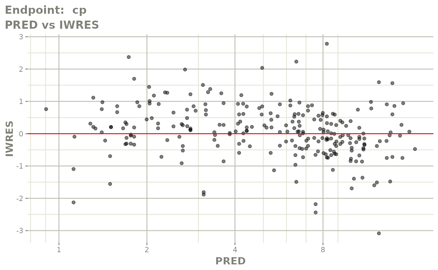
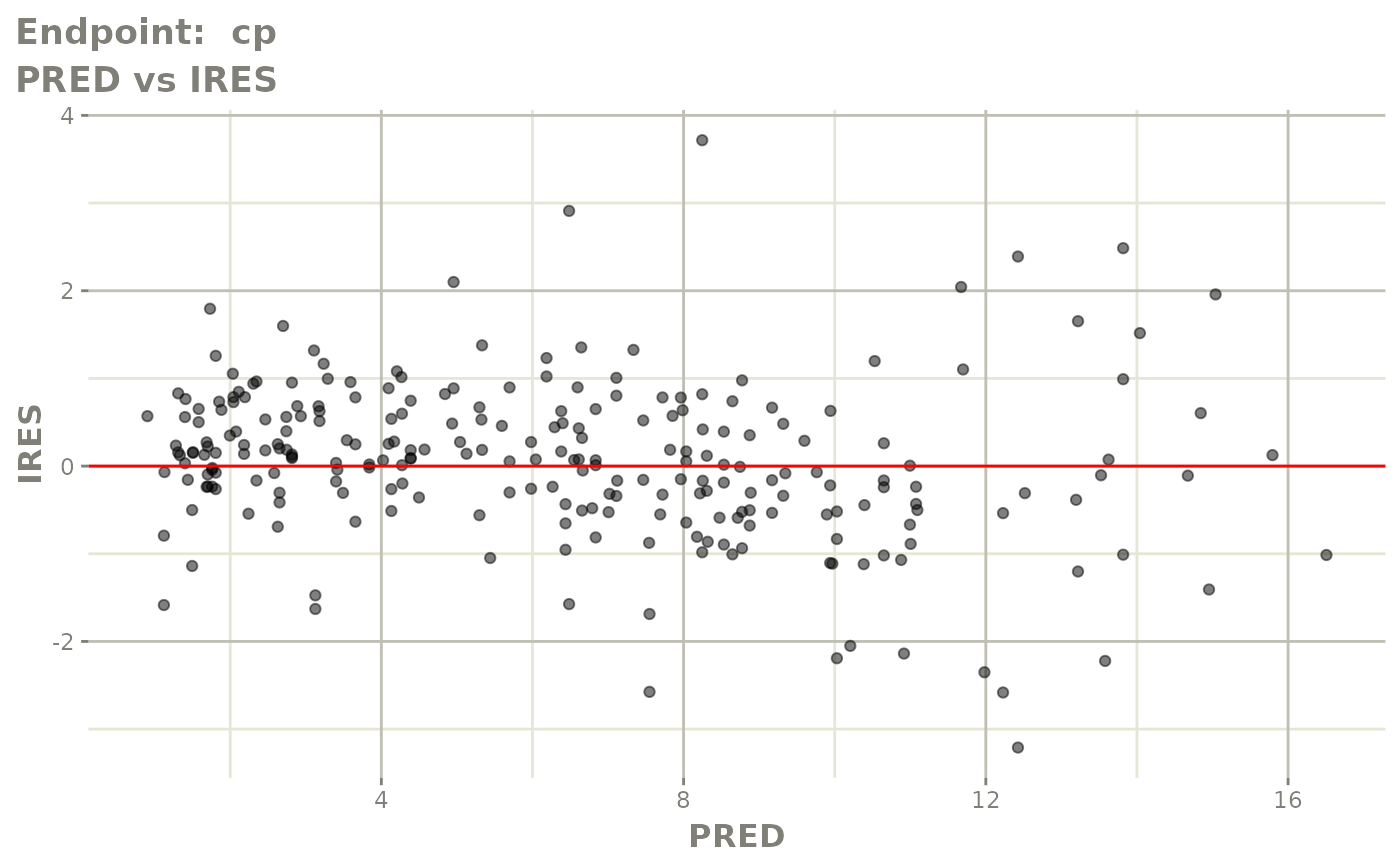
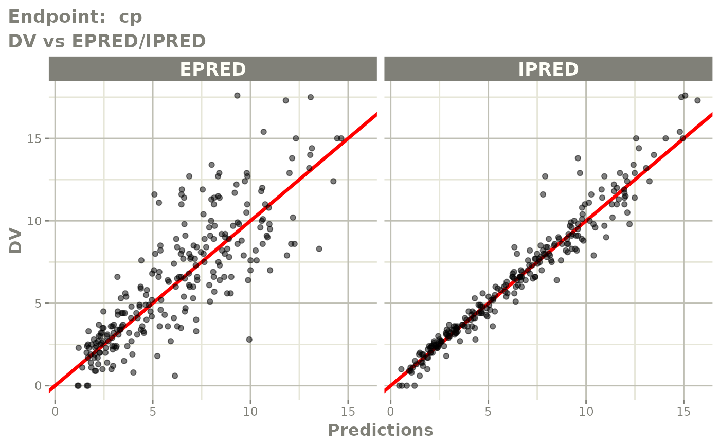
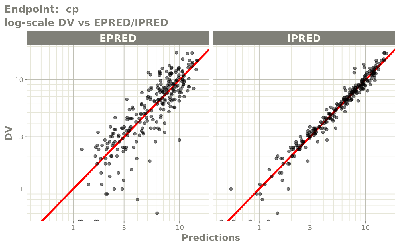
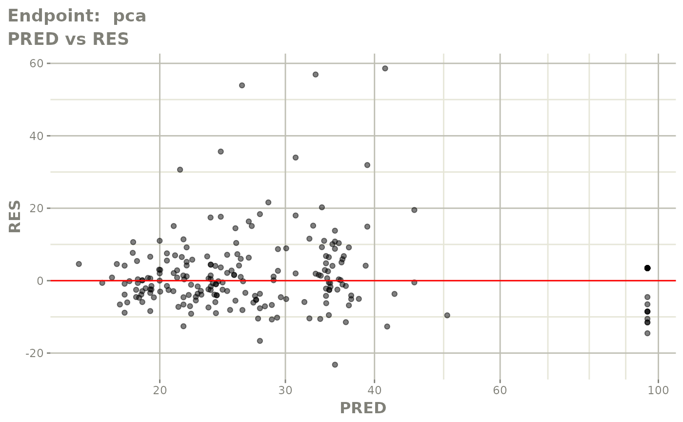
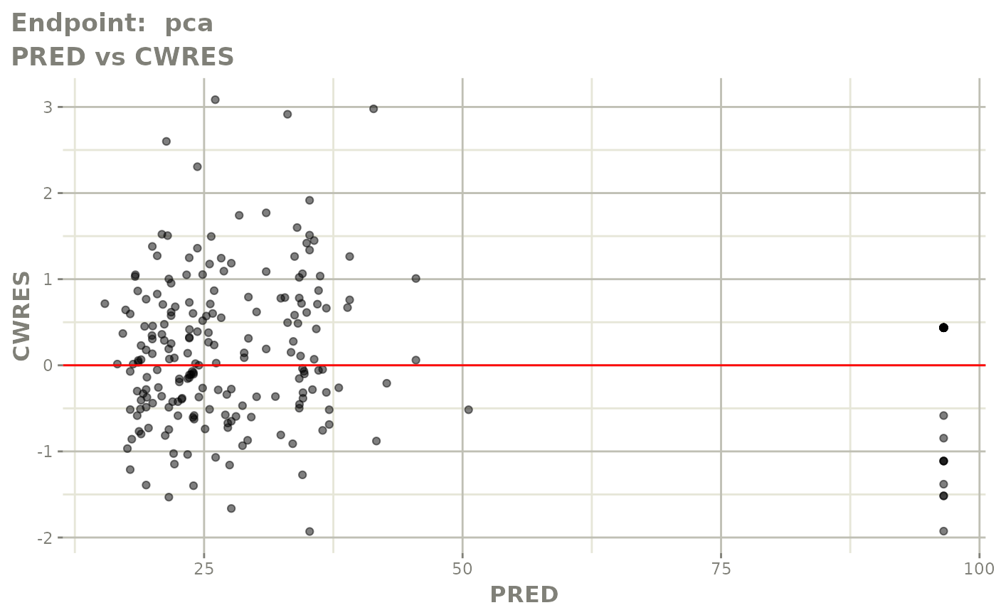
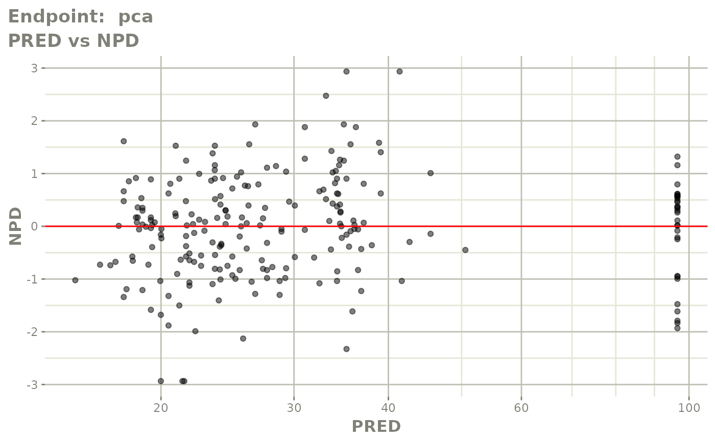
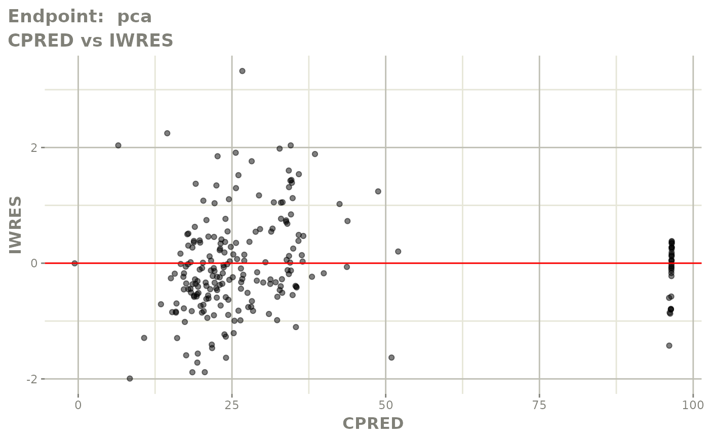
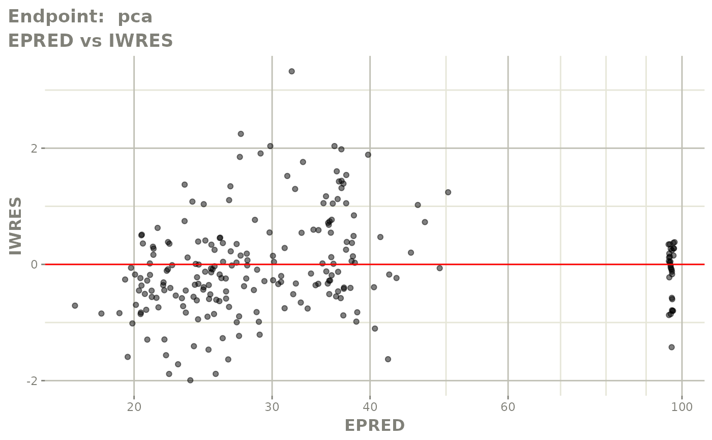
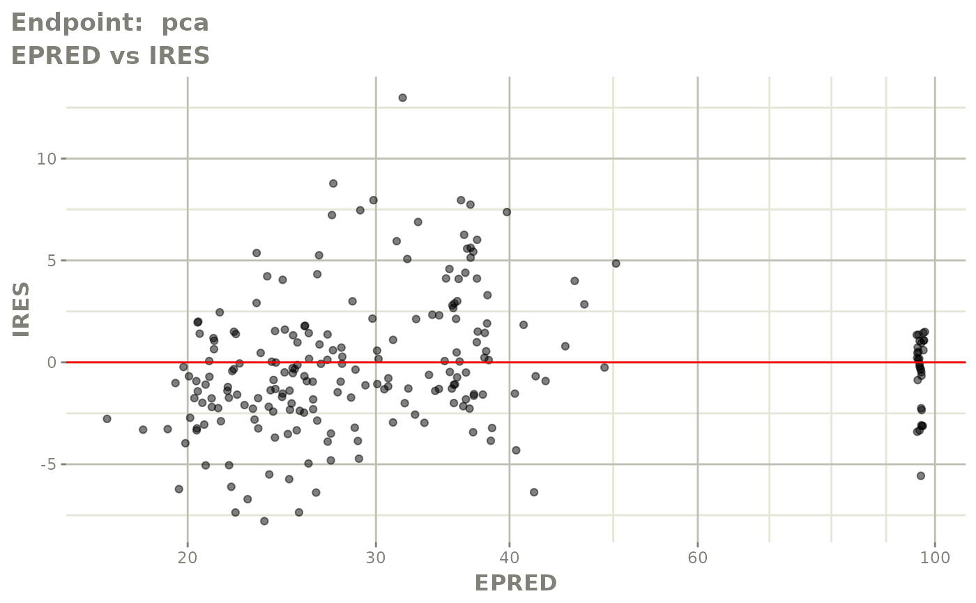
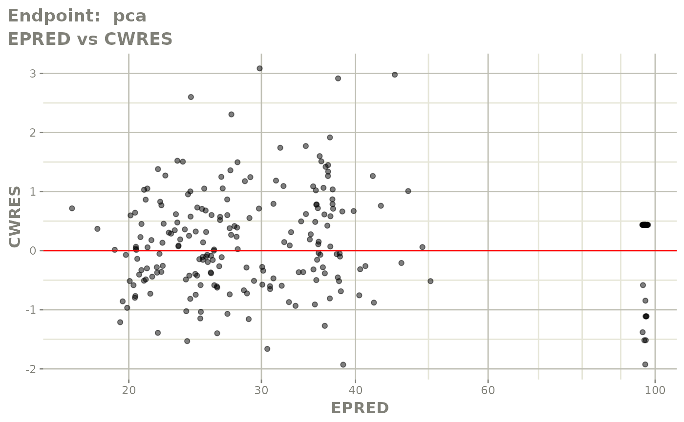
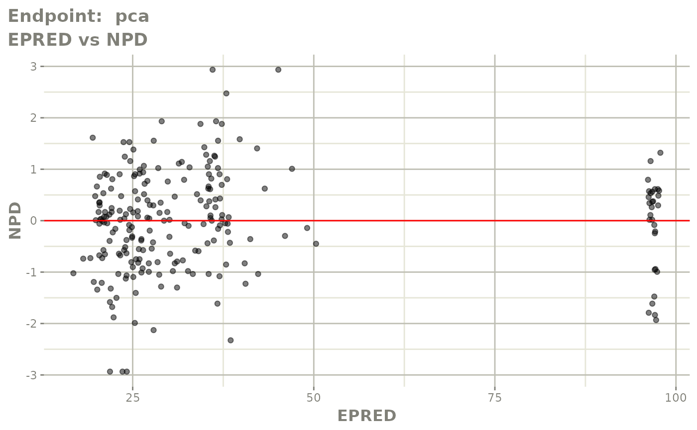
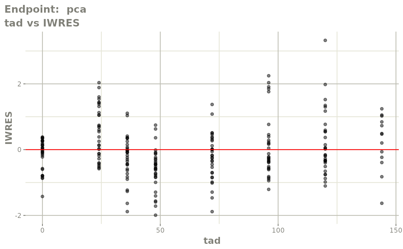
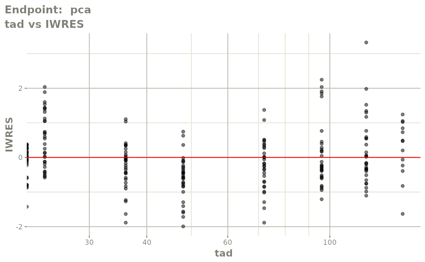
plot(fit.TOF)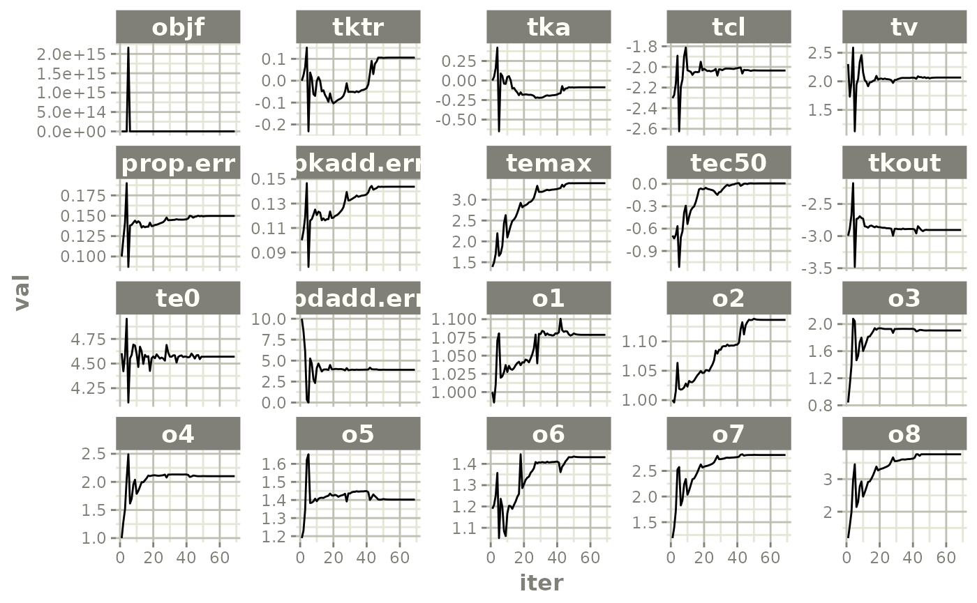


v1f <- nlmixr::vpc(fit.TOF, show=list(obs_dv=T), scales="free_y") +
  ylab("Warfarin Cp [mg/L] or PCA") +
  xlab("Time [h]")

v2f <- nlmixr::vpc(fit.TOF, show=list(obs_dv=T), pred_corr = TRUE) +
  ylab("Prediction Corrected Warfarin Cp [mg/L] or PCA") +
  xlab("Time [h]")

v1f / v2f