Nimotuzumab

Mirjam Trame

2022-03-26

nlmixr

This is an example of a complex model that can be estimated.

In the example below, a target-mediated drug disposition PK model for nimotuzumab is illustrated (Rodríguez-Vera et al. 2015).

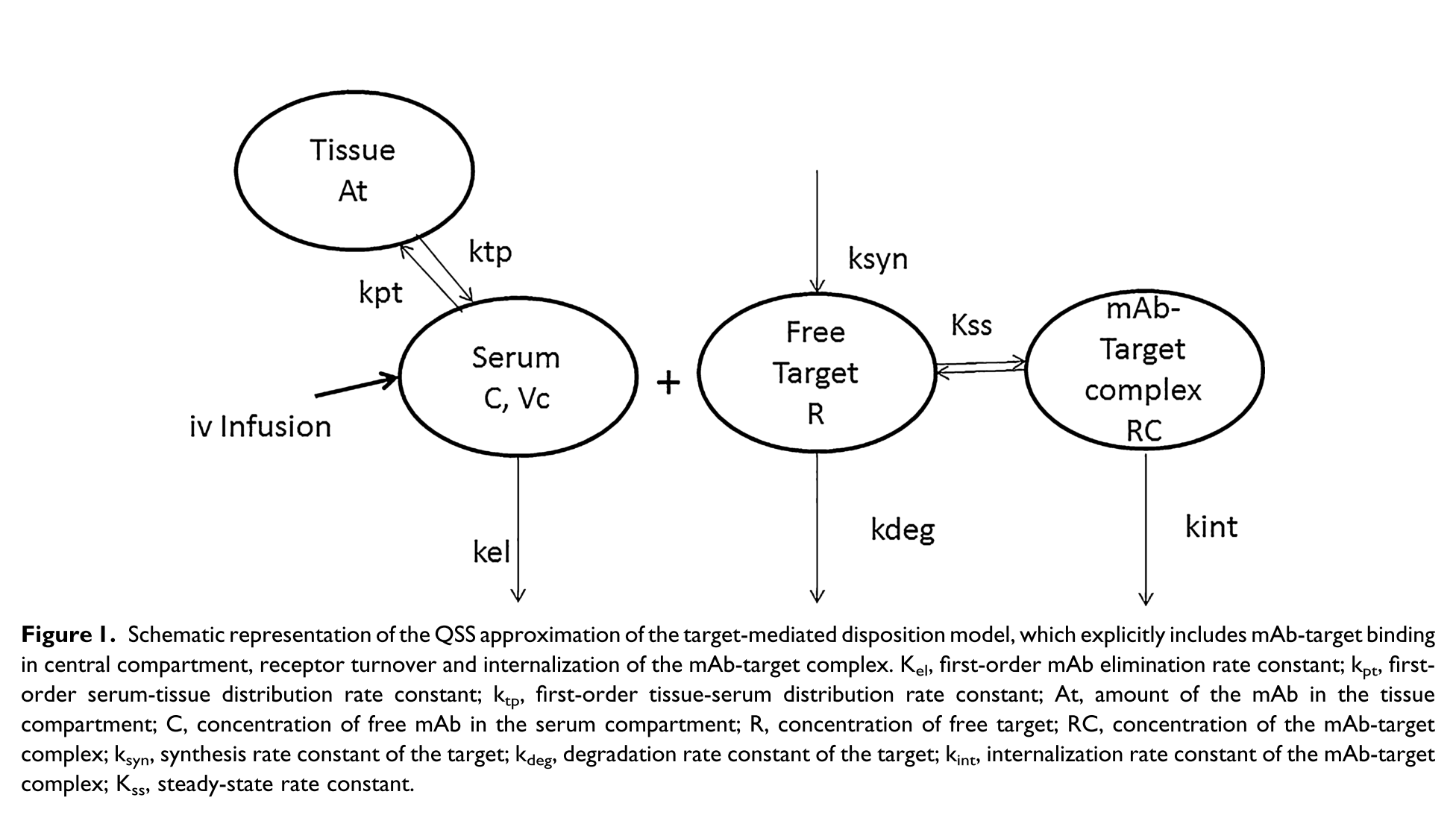
Model Schematic

nlmixr model

library(nlmixr)
library(xpose)
library(xpose.nlmixr)
library(ggplot2)

nimo <- function() {
  ini({
    ## Note that the UI can take expressions
    ## Also note that these initial estimates should be provided on the log-scale
    tcl <- log(0.001)
    tv1 <- log(1.45)
    tQ <- log(0.004)
    tv2 <- log(44)
    tkss <- log(12)
    tkint <- log(0.3)
    tksyn <- log(1)
    tkdeg <- log(7)
    ## Initial estimates should be high for SAEM ETAs
    eta.cl  ~ 2
    eta.v1  ~ 2
    eta.kss ~ 2
    ##  Also true for additive error (also ignored in SAEM)
    add.err <- 10
  })
  model({
    cl <- exp(tcl + eta.cl)
    v1 <- exp(tv1 + eta.v1)
    Q  <- exp(tQ)
    v2 <- exp(tv2)
    kss <- exp(tkss + eta.kss)
    kint <- exp(tkint)
    ksyn <- exp(tksyn)
    kdeg <- exp(tkdeg)

    k <- cl/v1
    k12 <- Q/v1
    k21 <- Q/v2

    eff(0) <- ksyn/kdeg ##initializing compartment

    ## Concentration is calculated
    conc = 0.5*(central/v1-eff-kss)+0.5*sqrt((central/v1-eff-kss)**2+4*kss*central/v1)

    d/dt(central)  = -(k+k12)*conc*v1+k21*peripheral-kint*eff*conc*v1/(kss+conc)
    d/dt(peripheral) = k12*conc*v1-k21*peripheral  ##Free Drug second compartment amount
    d/dt(eff) = ksyn - kdeg*eff - (kint-kdeg)*conc*eff/(kss+conc)

    IPRED=log(conc)

    IPRED ~ add(add.err)
  })
}

Fit

load("nimoData.rda")
fit <- nlmixr(nimo, nimoData, est="saem", control=list(print=0),
              table=list(cwres=TRUE, npde=TRUE))
#> [====|====|====|====|====|====|====|====|====|====] 0:00:00 
#> 
#> [====|====|====|====|====|====|====|====|====|====] 0:00:03 
#> 
#> [====|====|====|====|====|====|====|====|====|====] 0:00:04 
#> 
#> [====|====|====|====|====|====|====|====|====|====] 0:00:00 
#> 
#> [====|====|====|====|====|====|====|====|====|====] 0:00:00

Goodness of fit Plots

## Add cwres/npde after fit
fit  <- fit %>% addCwres() %>% addNpde();
## Since it is already there it doesn't actually change anything.


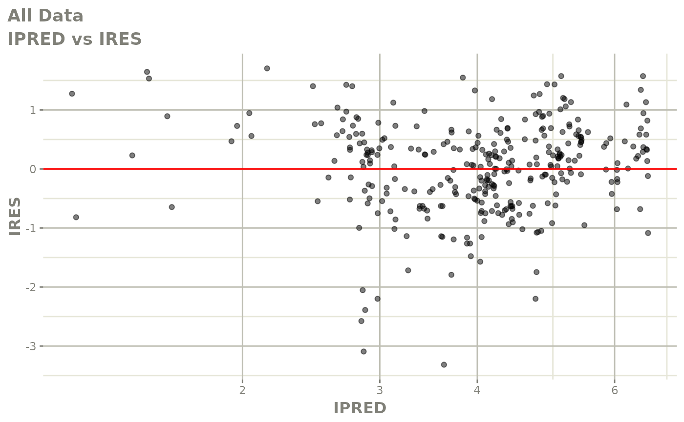
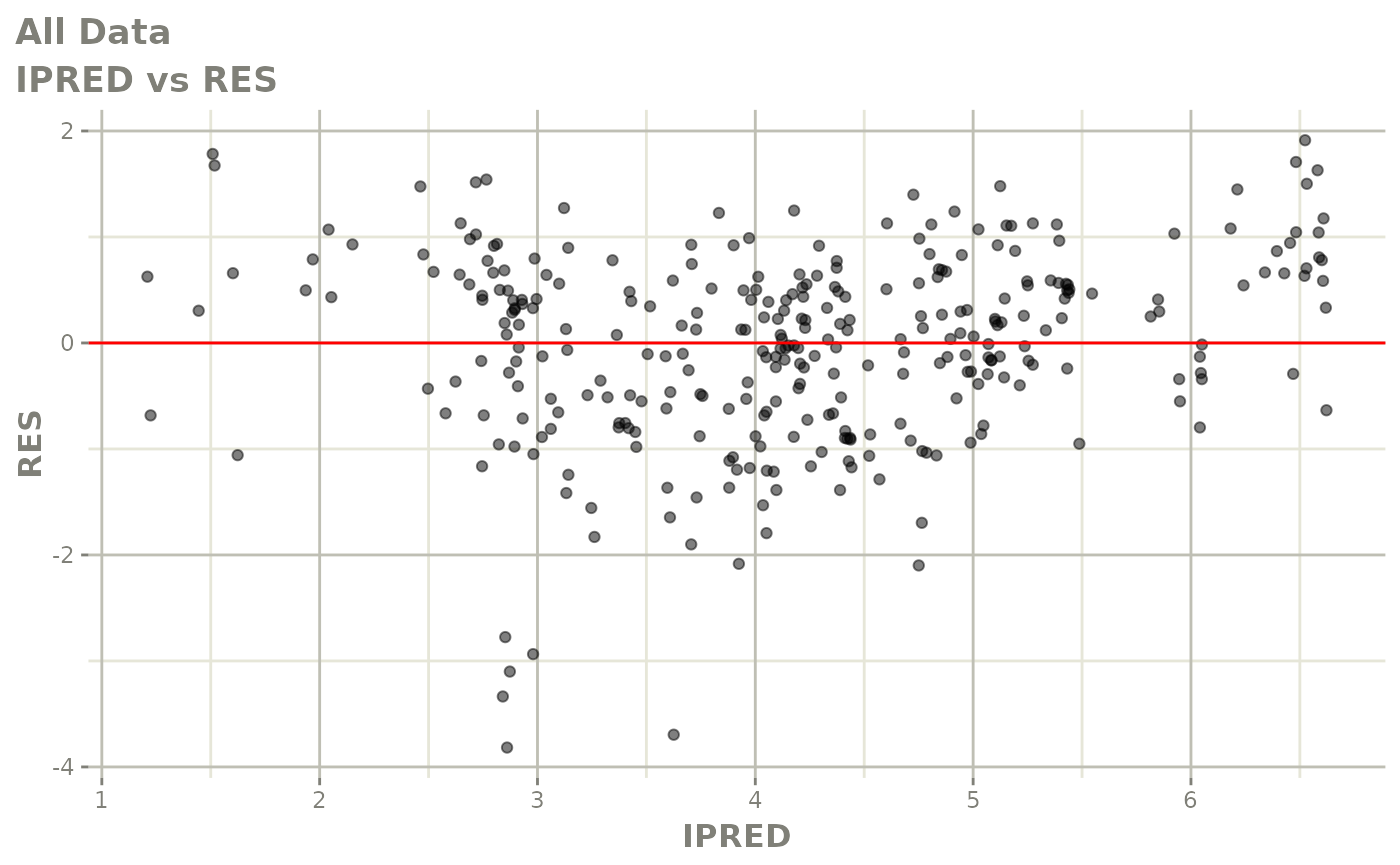
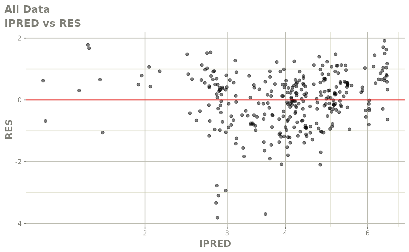
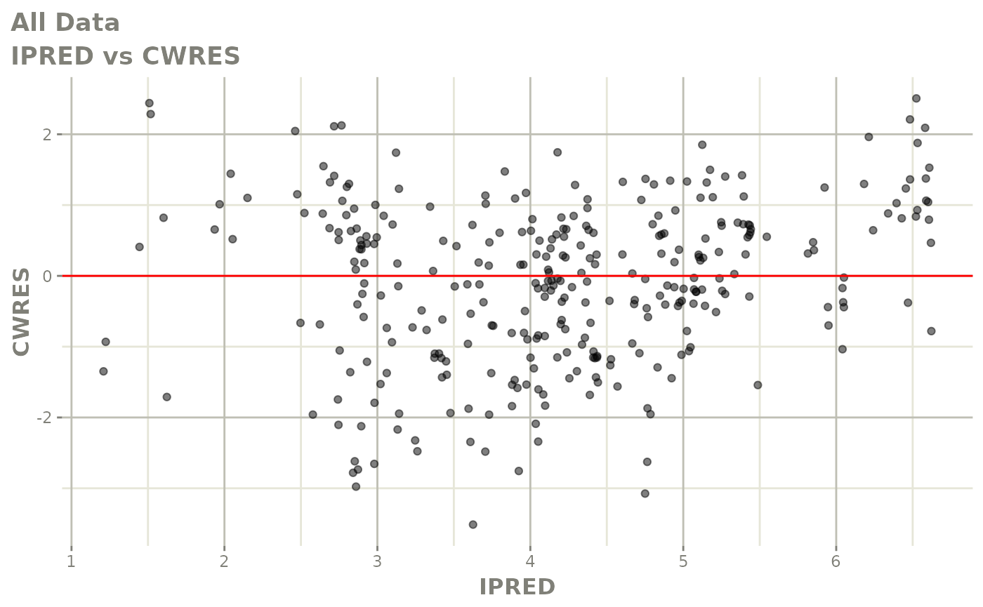
##Goodness-of-fit plots

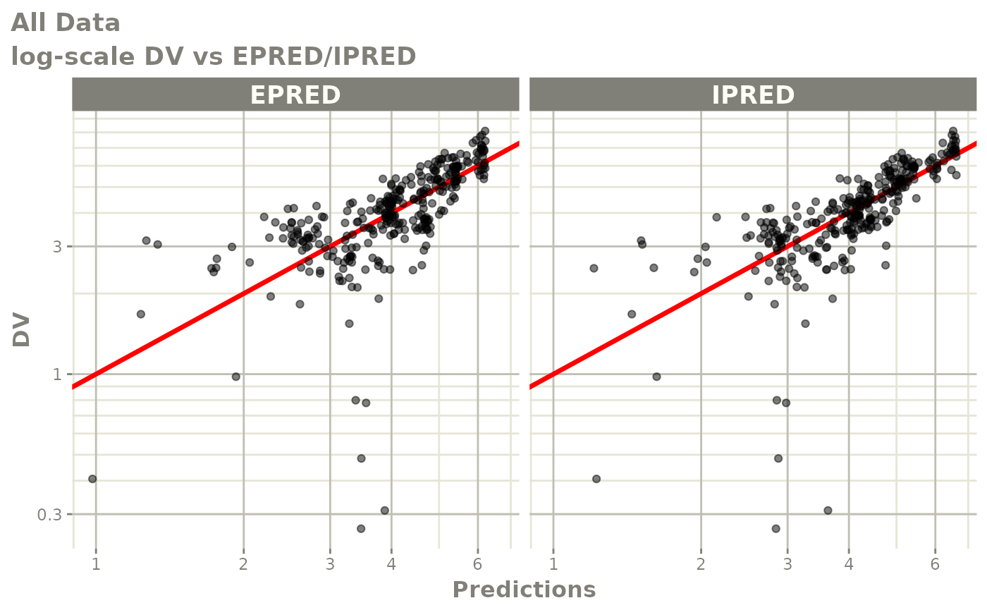
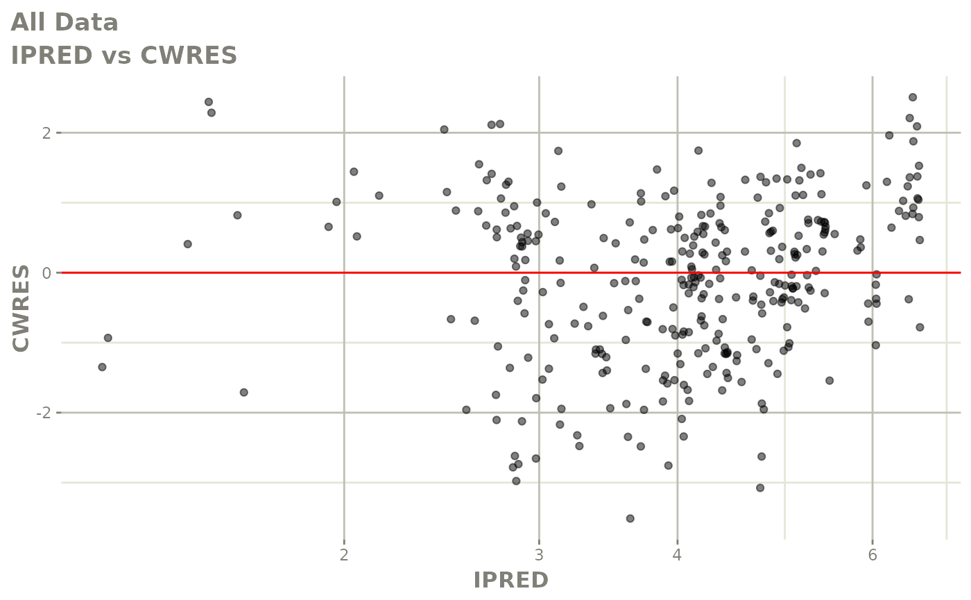
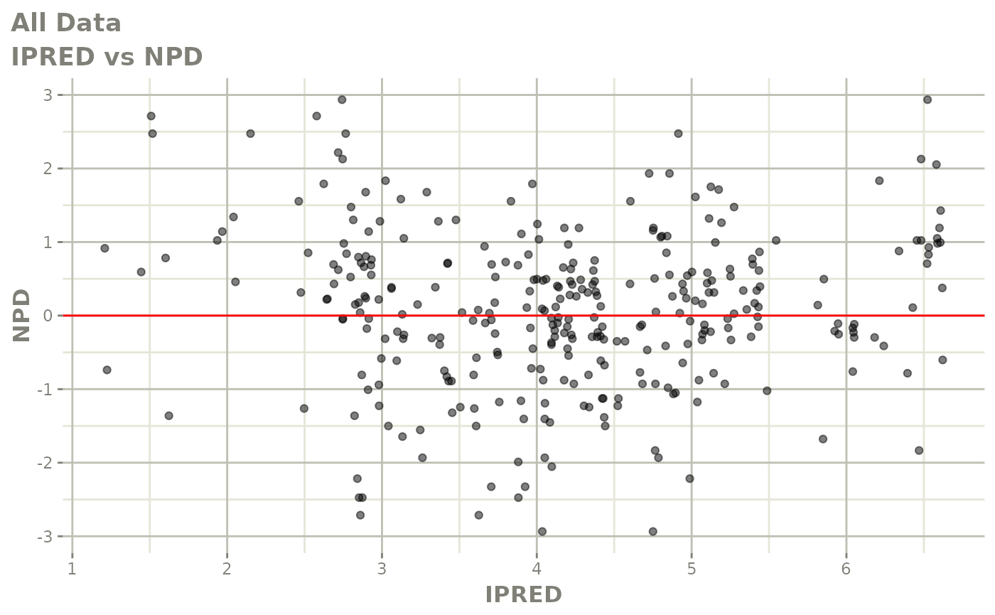
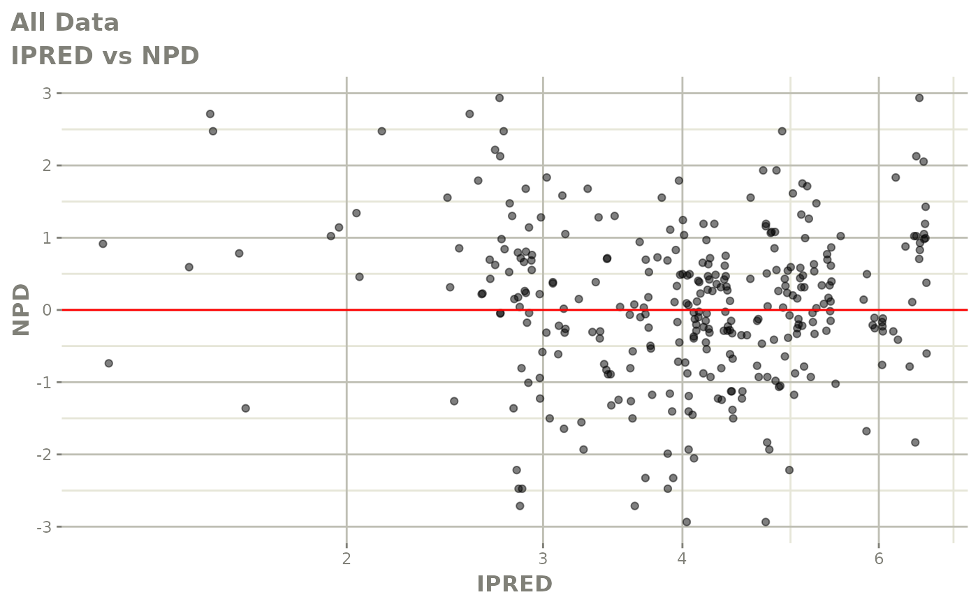
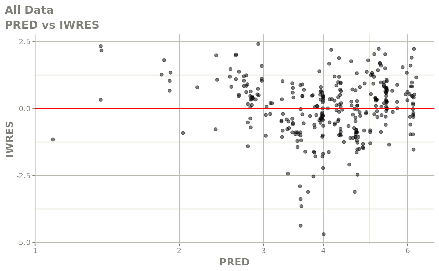
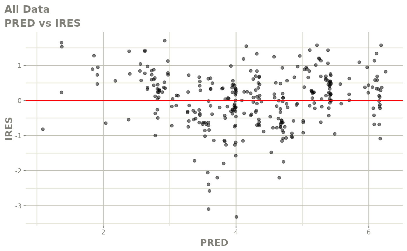
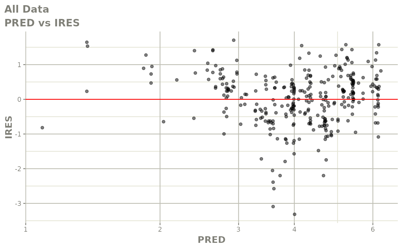
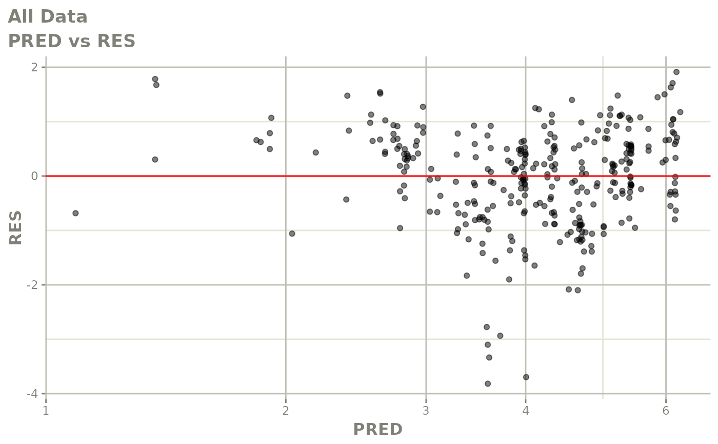
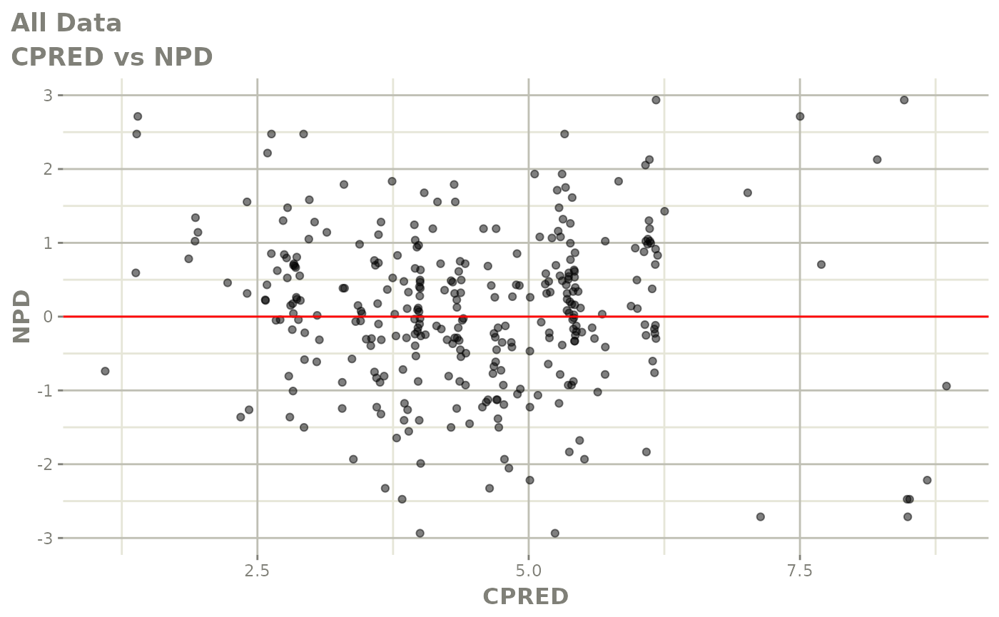
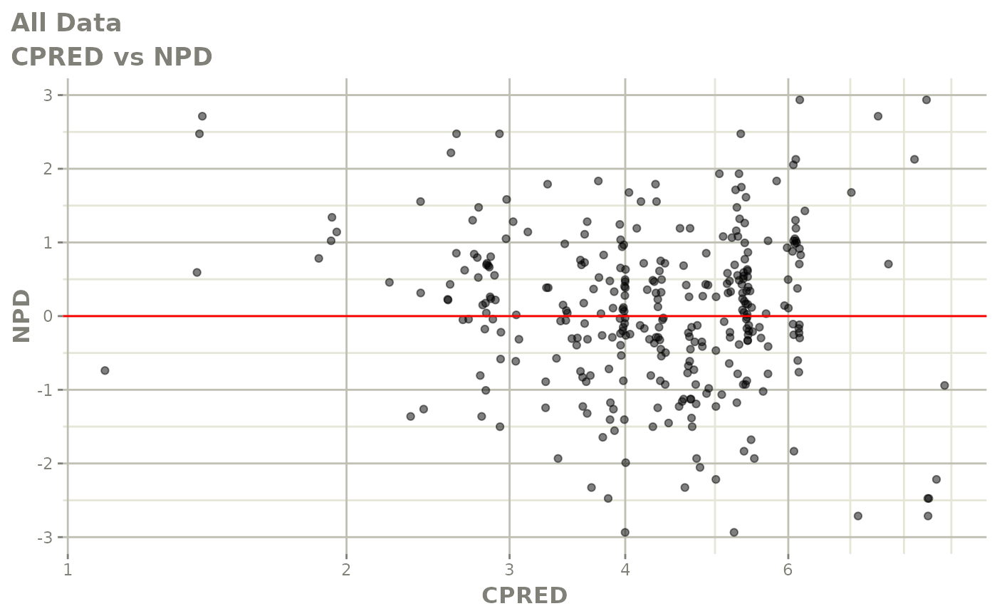
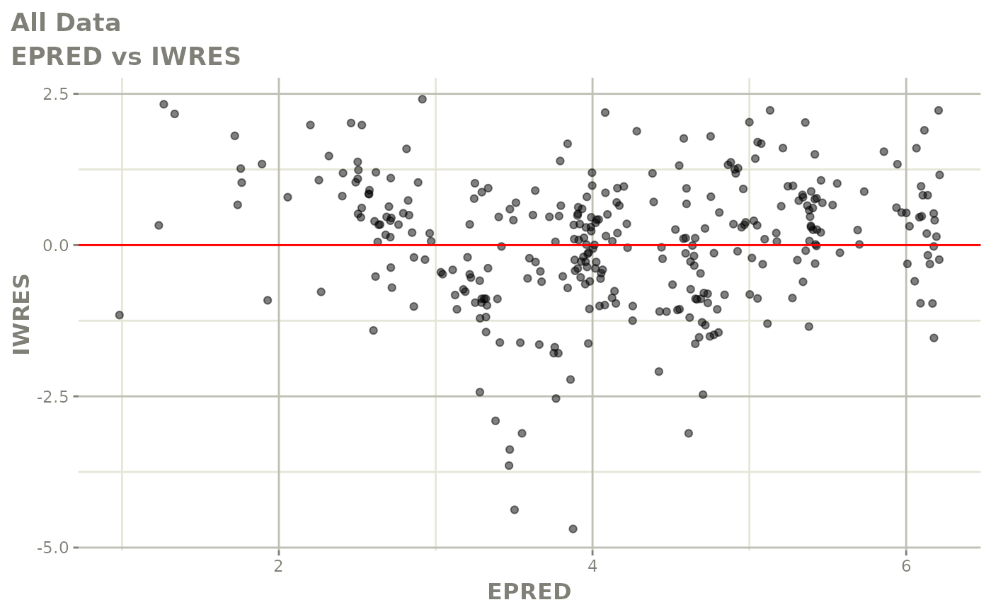
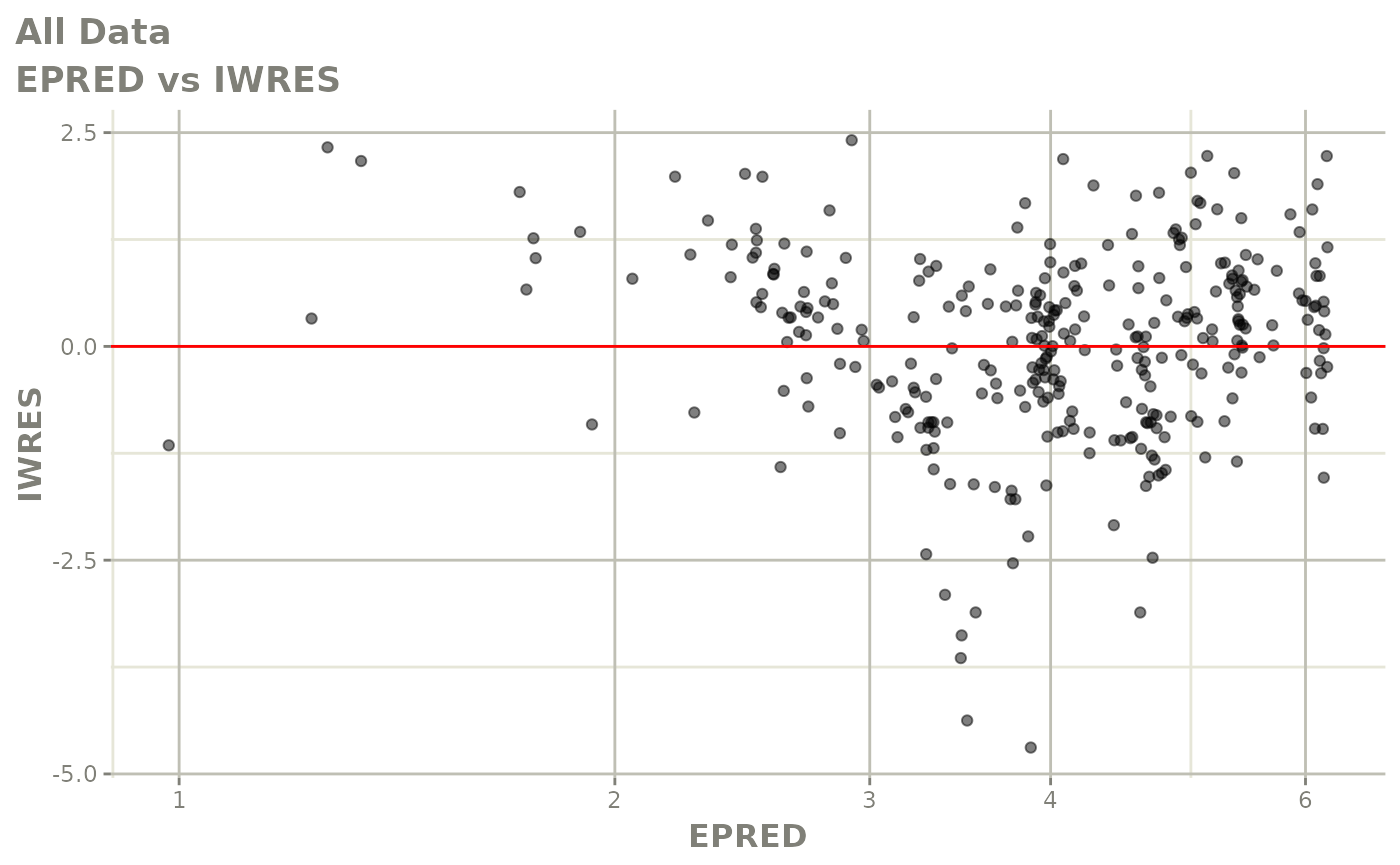
plot(fit); ## Standard nlmixr plots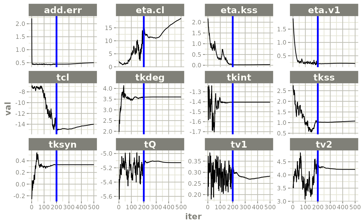

################################################################################
## Xpose plots; Need to print otherwise running a script won't
## show xpose plots
################################################################################
xpdb <- xpose_data_nlmixr(fit) ## first convert to nlmixr object

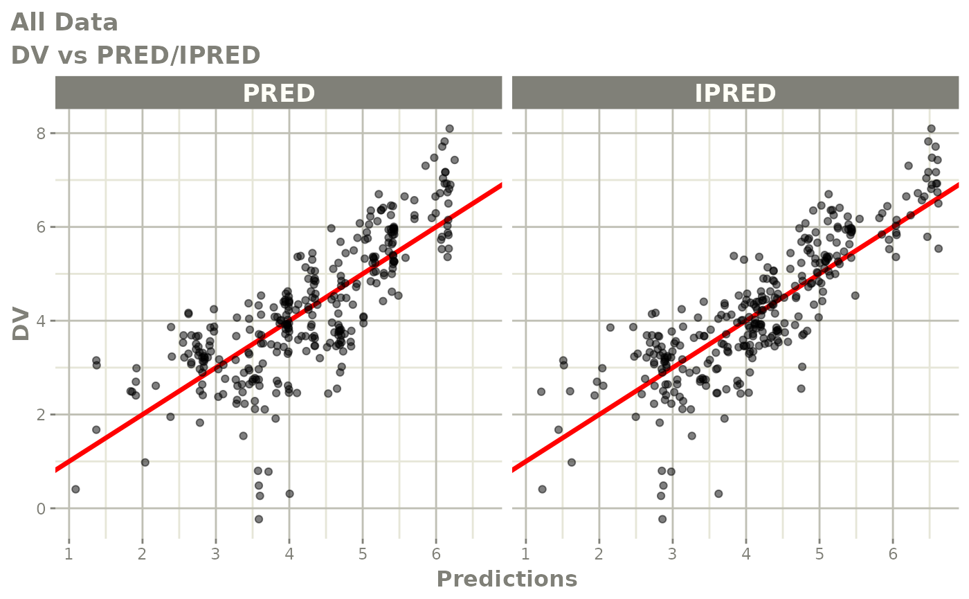
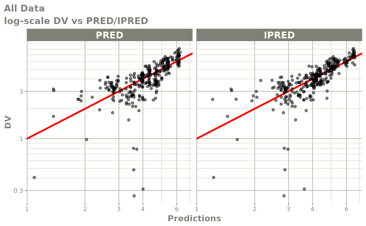
print(dv_vs_pred(xpdb) +
      ylab("Observed Nimotuzumab Concentrations (ug/mL)") +
      xlab("Population Predicted Nimotuzumab Concentrations (ug/mL)"))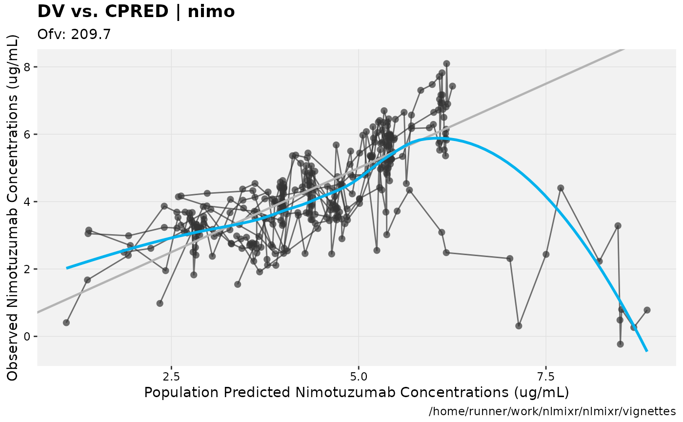

print(dv_vs_ipred(xpdb) +
      ylab("Observed Nimotuzumab Concentrations (ug/mL)") +
      xlab("Individual Predicted Nimotuzumab Concentrations (ug/mL)"))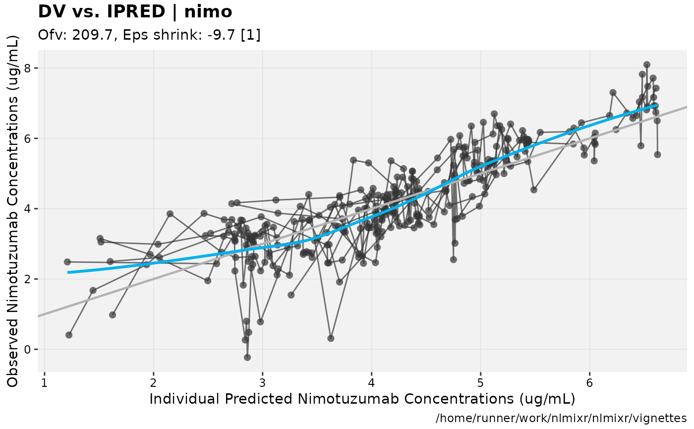

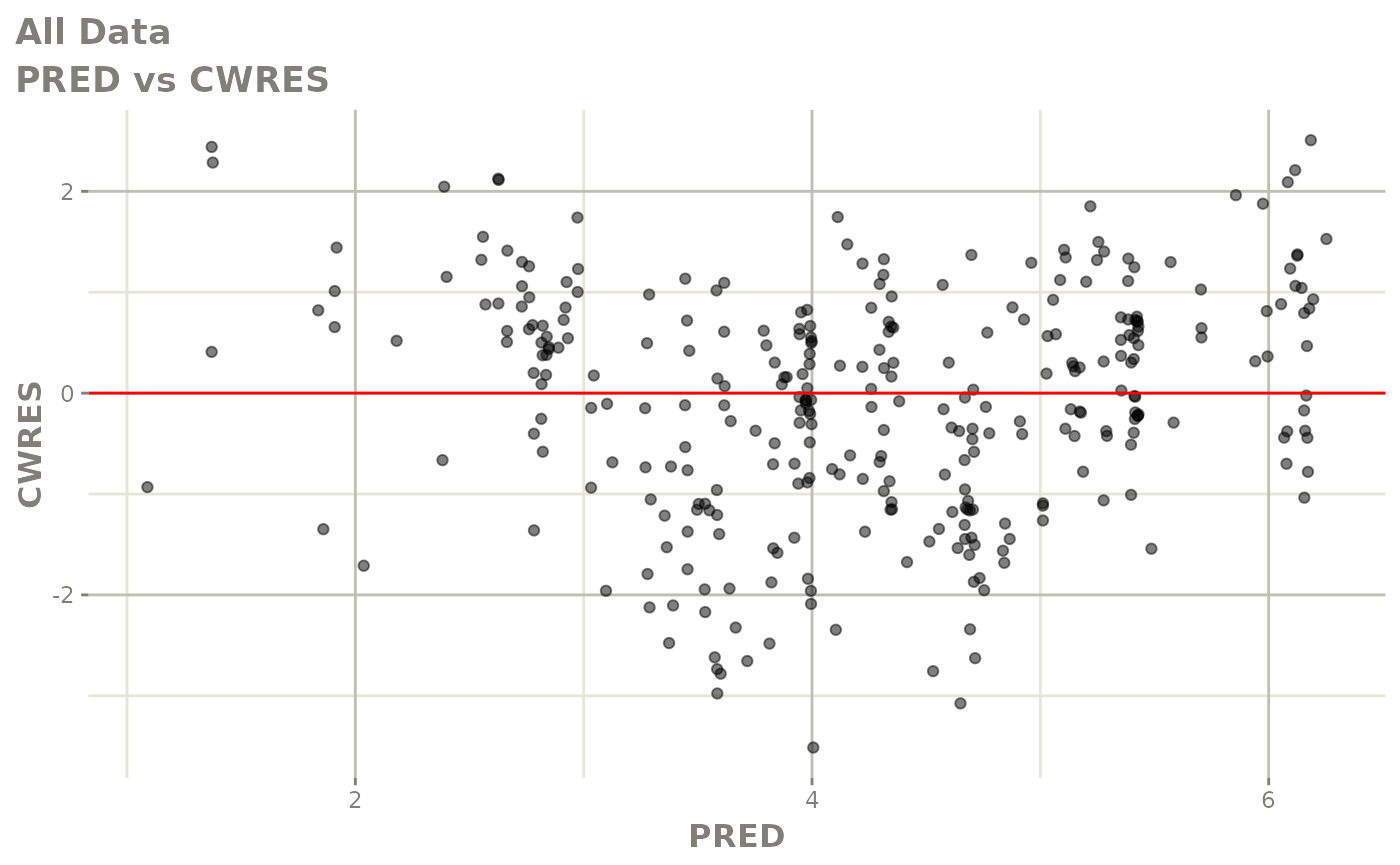
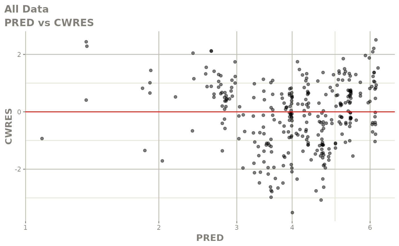
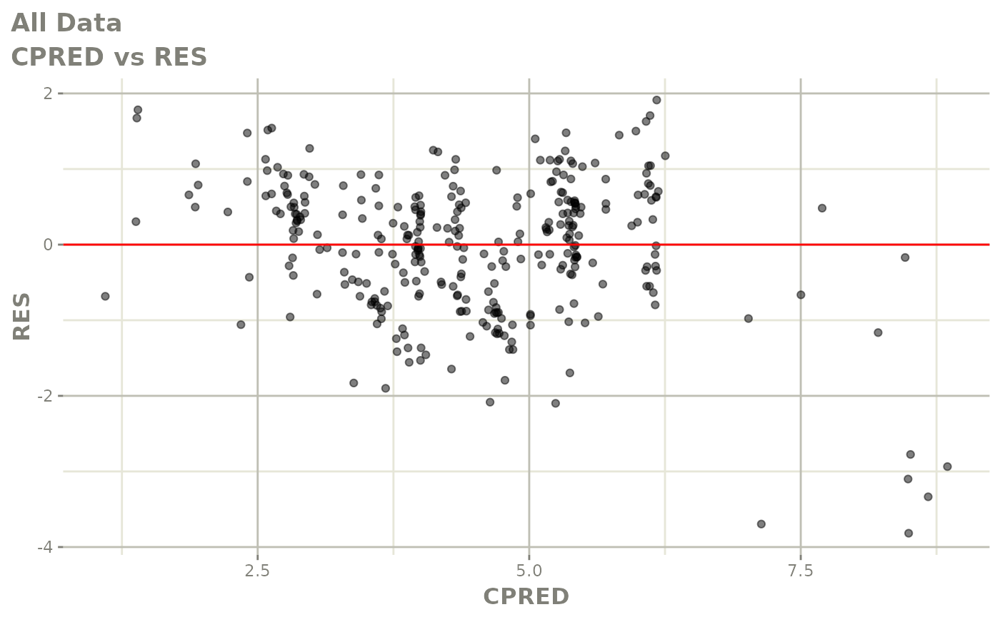
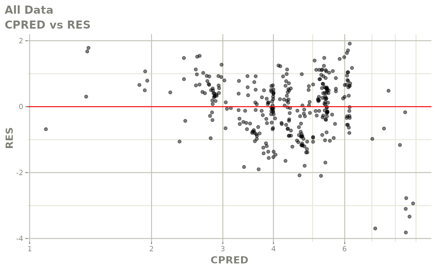
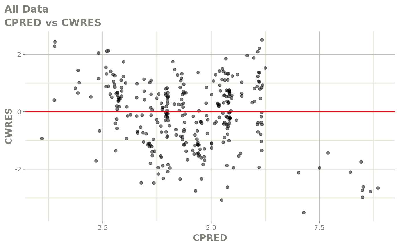
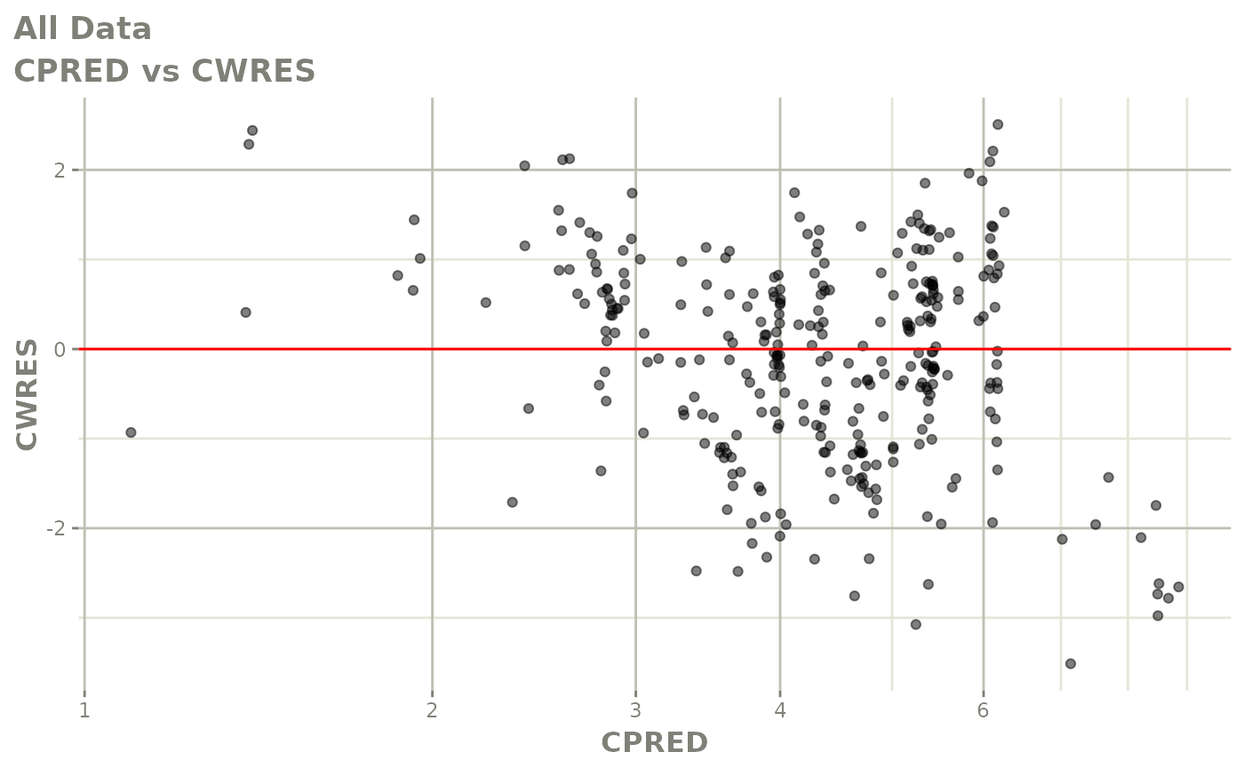
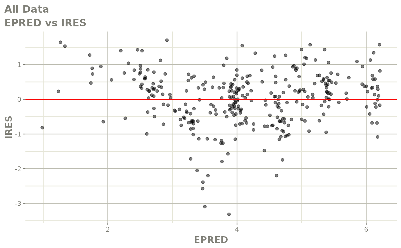
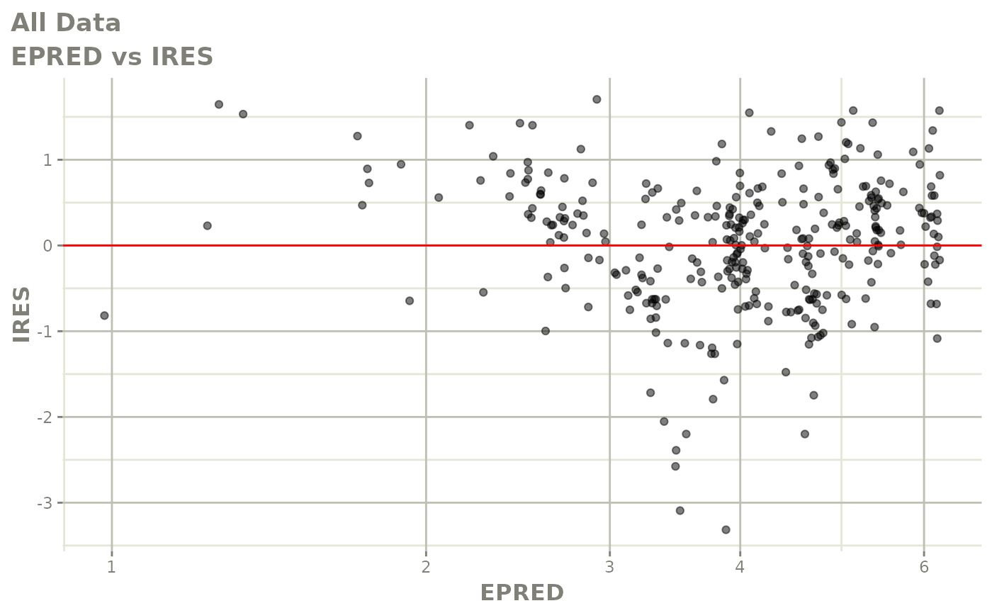
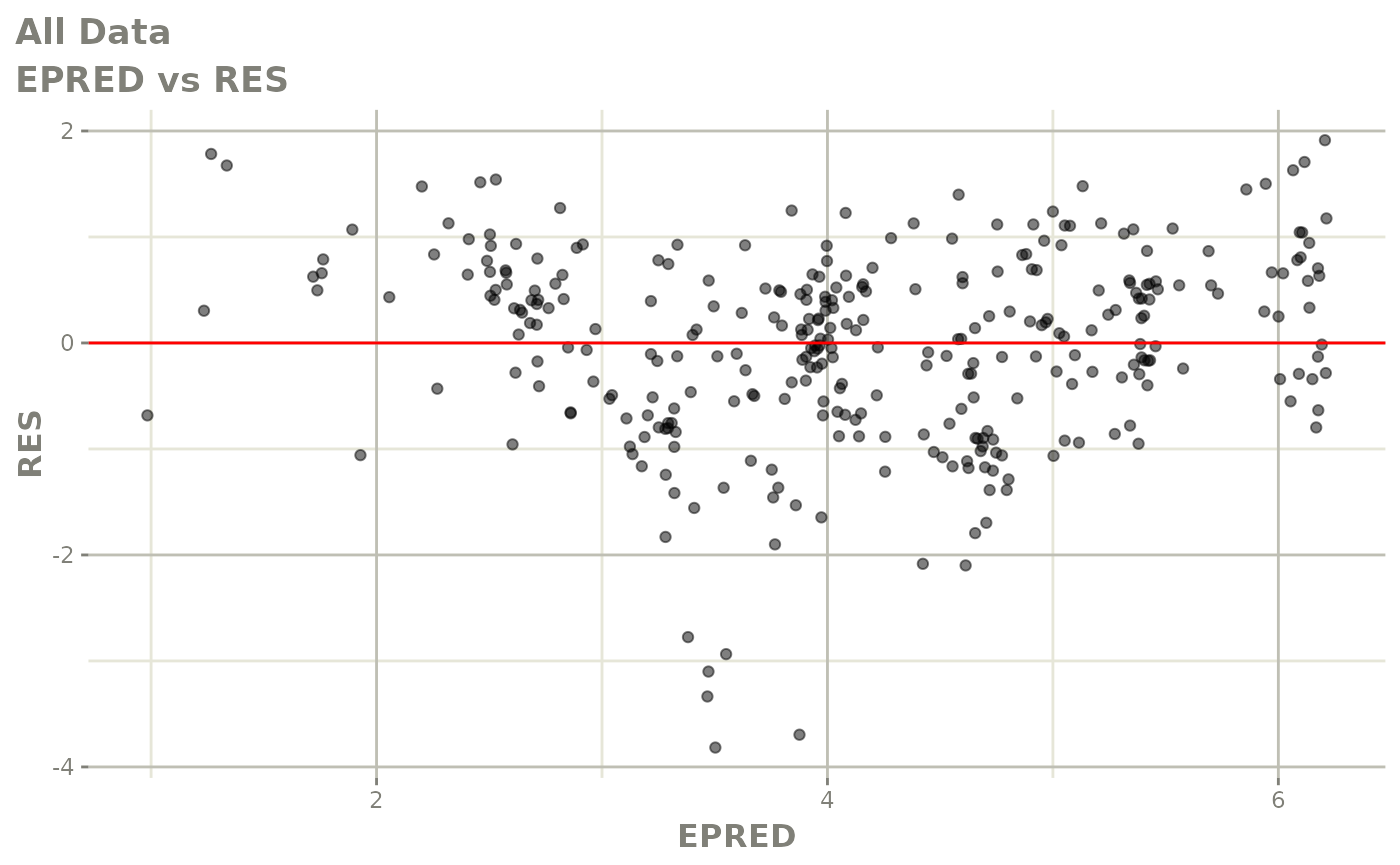
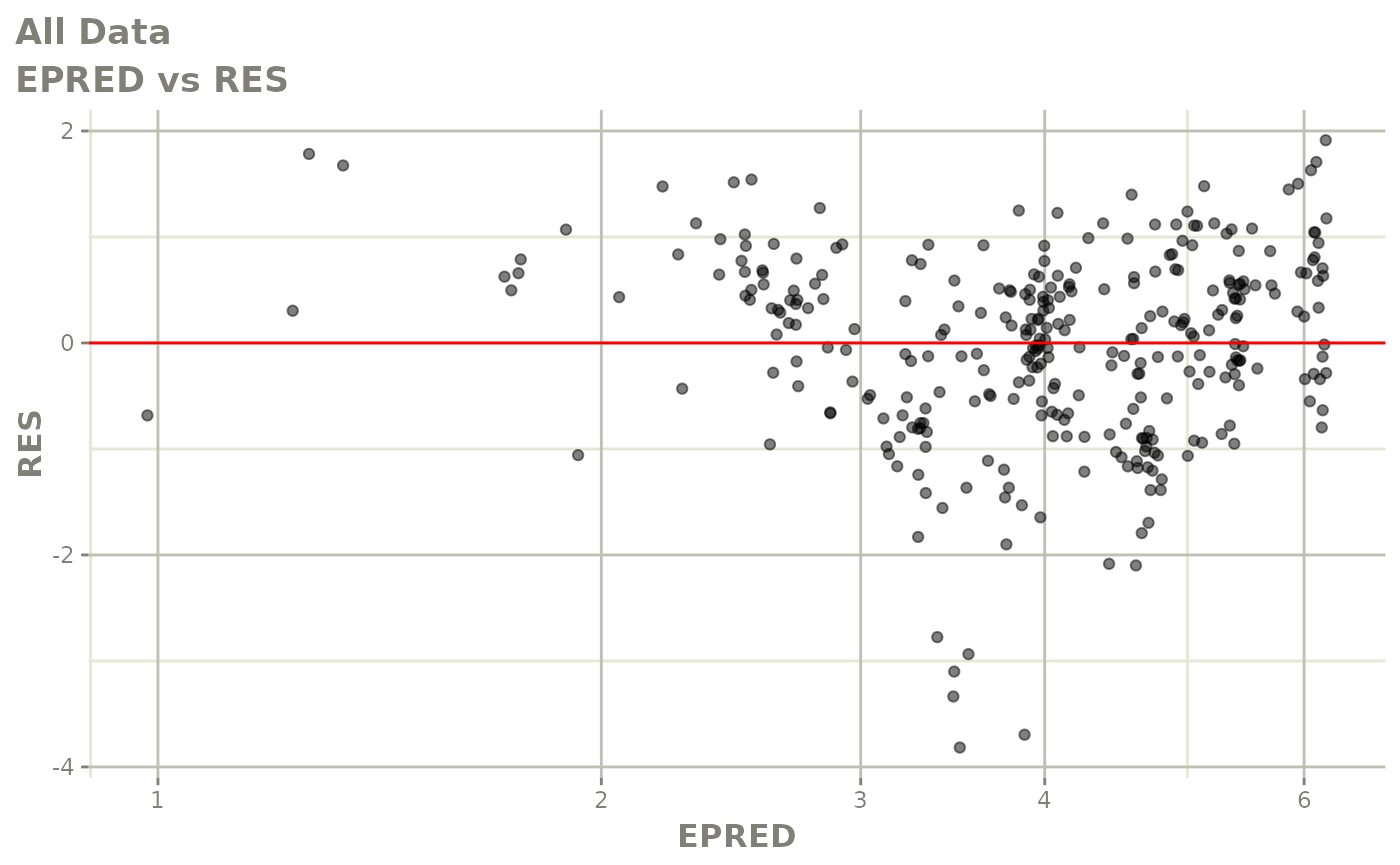
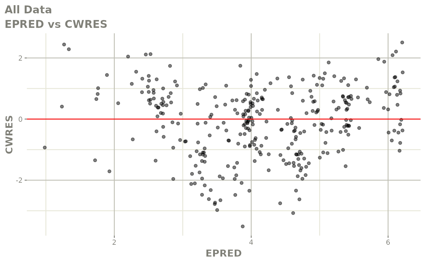
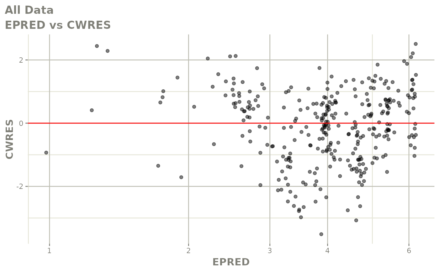
print(res_vs_pred(xpdb) +
      ylab("Conditional Weighted Residuals") +
      xlab("Population Predicted Nimotuzumab Concentrations (ug/mL)"))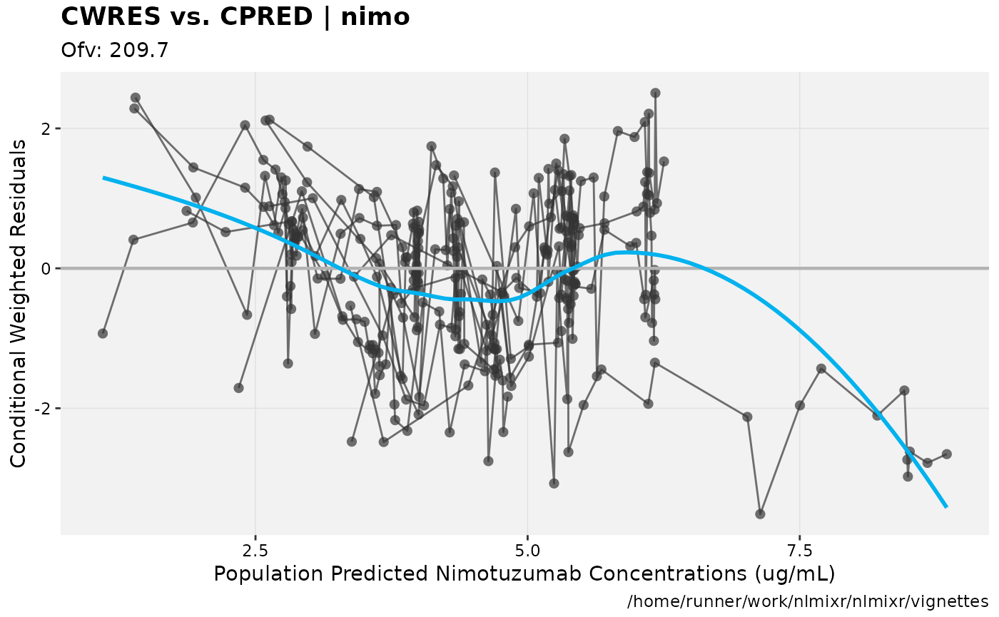

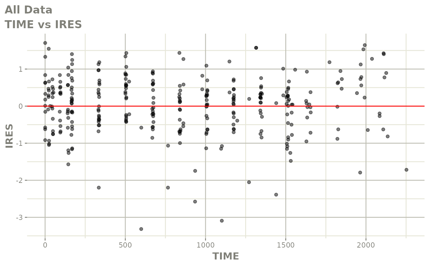
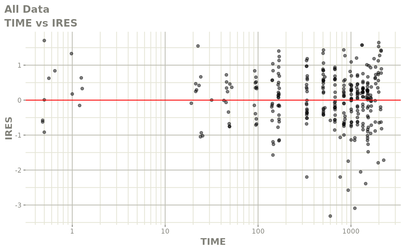
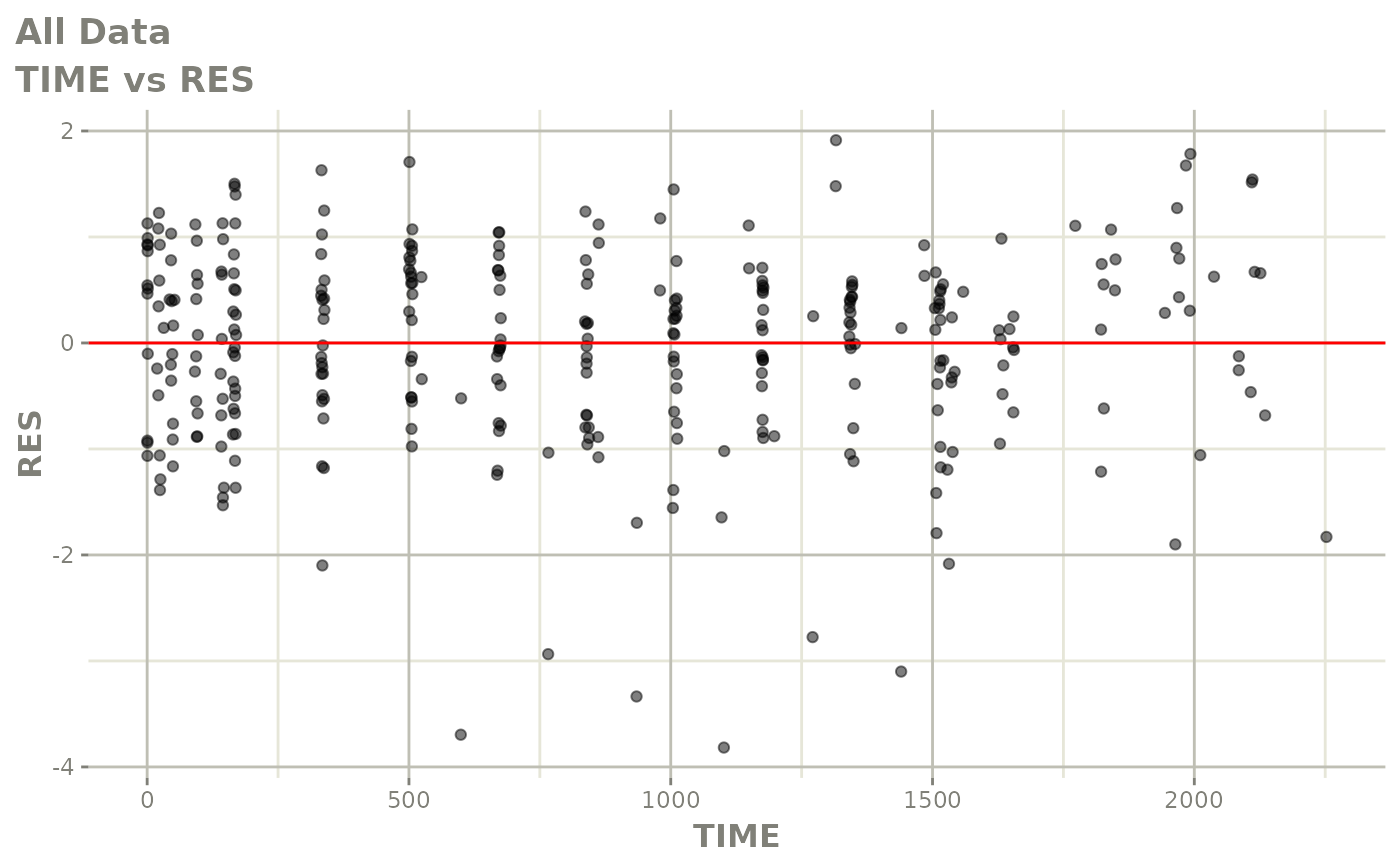
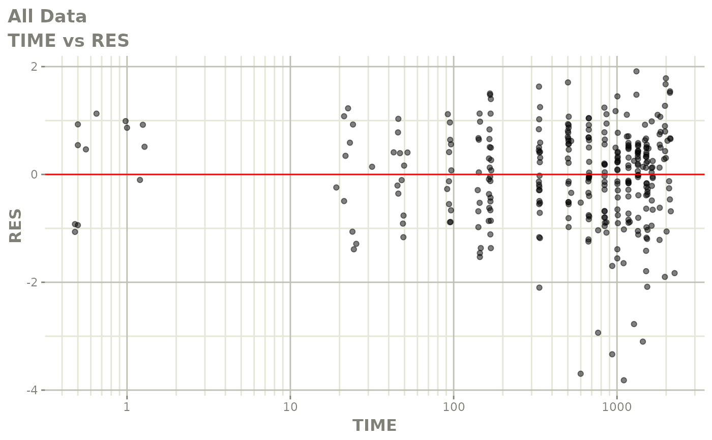
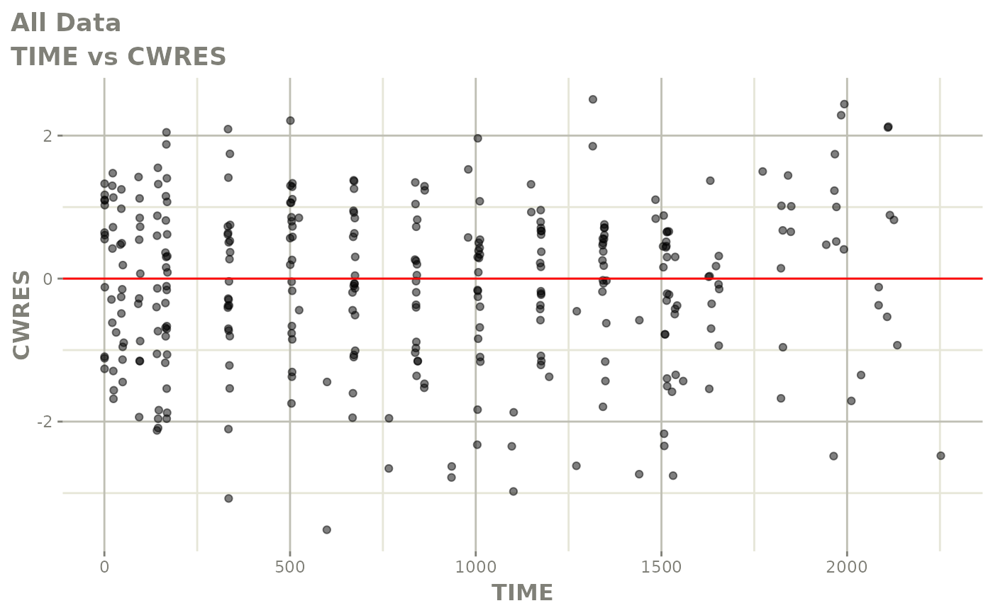
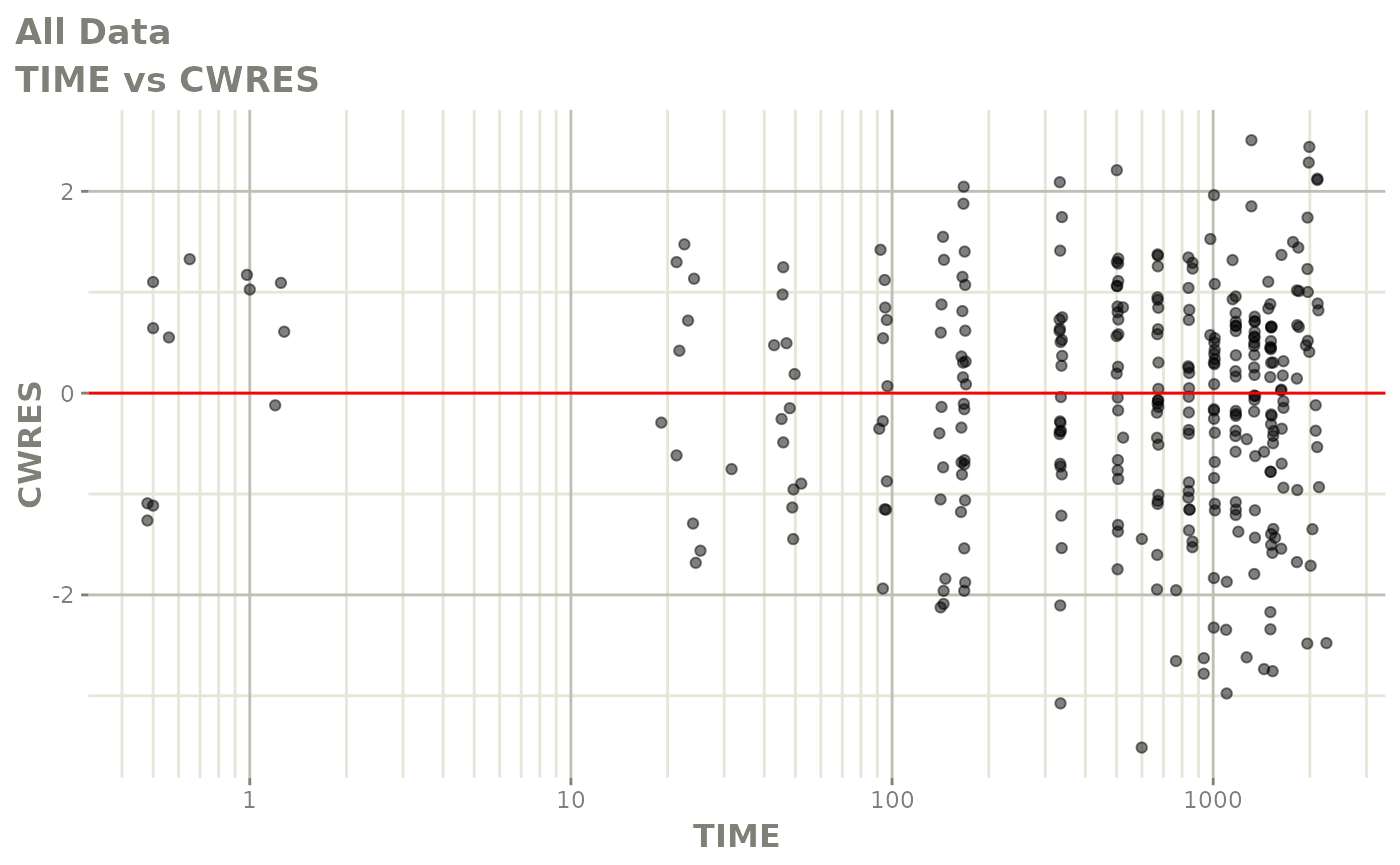
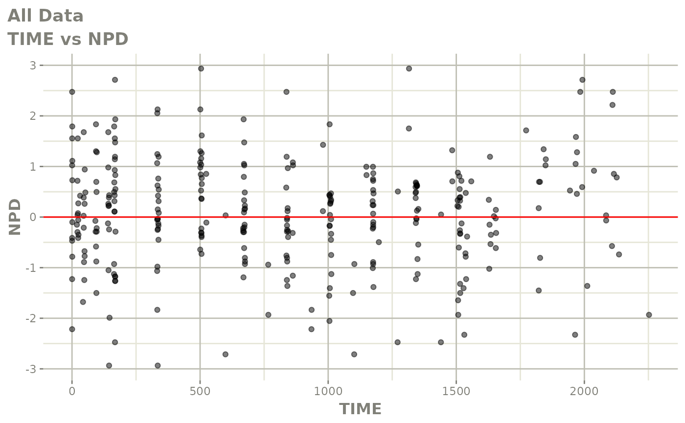
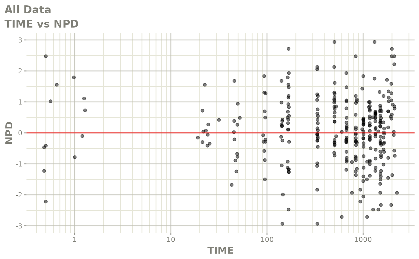
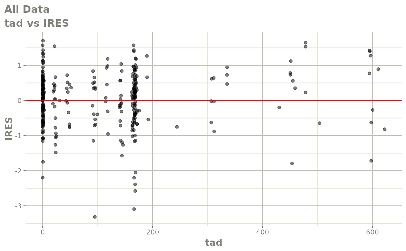
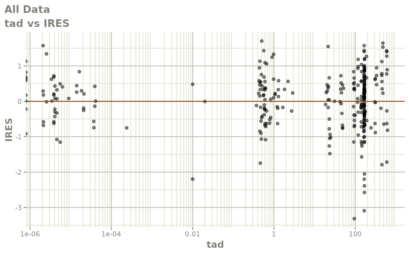
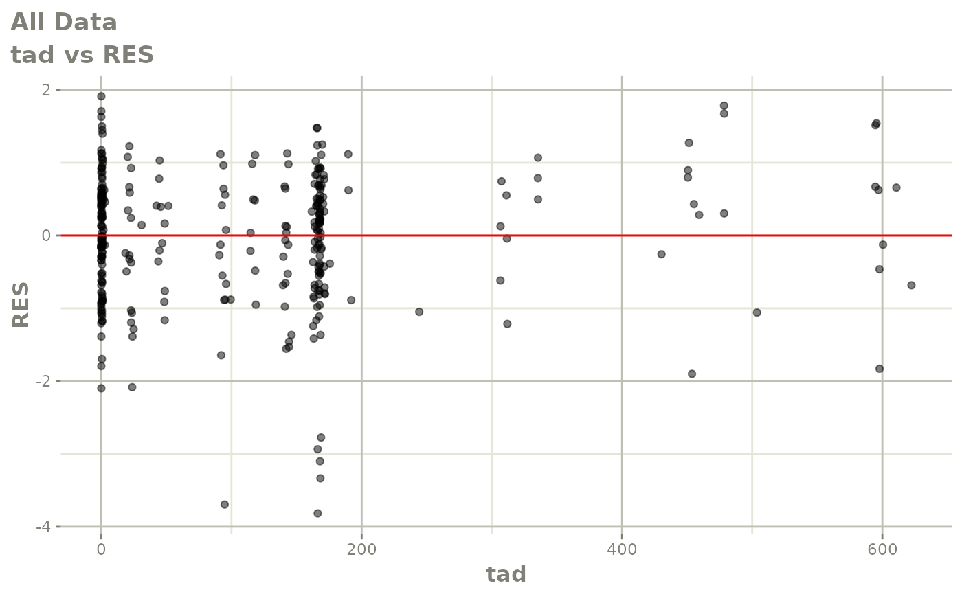
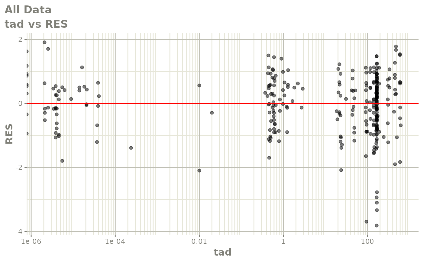
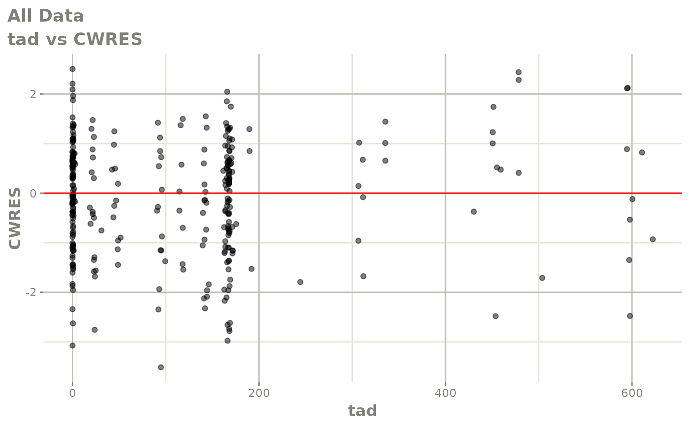
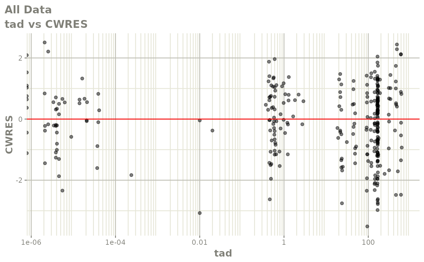
print(res_vs_idv(xpdb) +
      ylab("Conditional Weighted Residuals") +
      xlab("Time (h)"))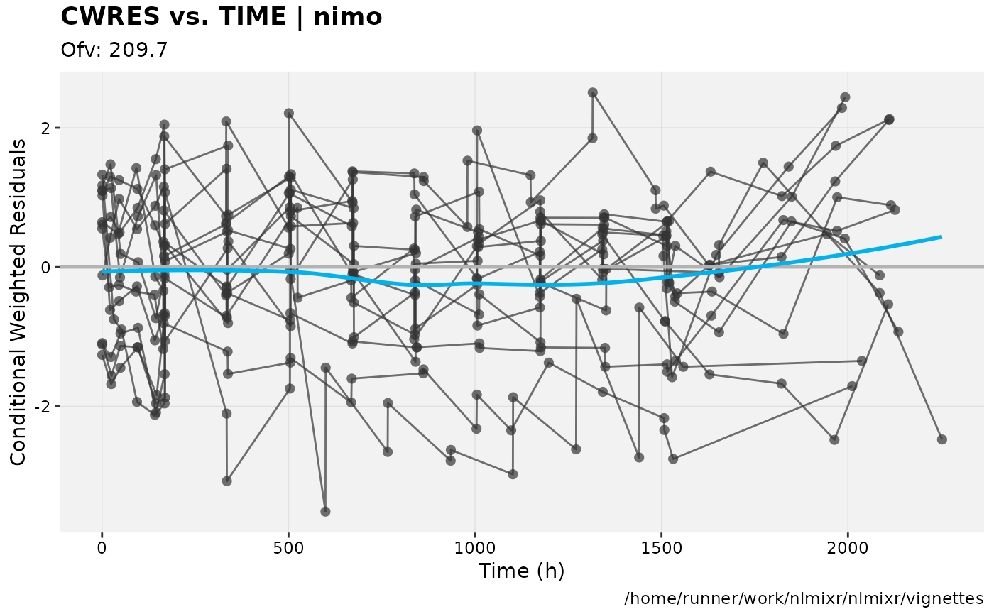

print(prm_vs_iteration(xpdb))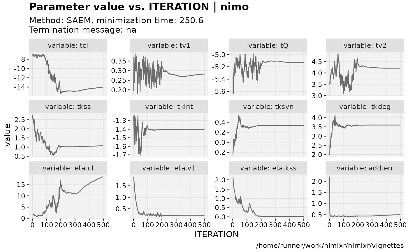

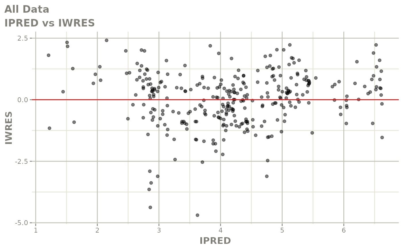
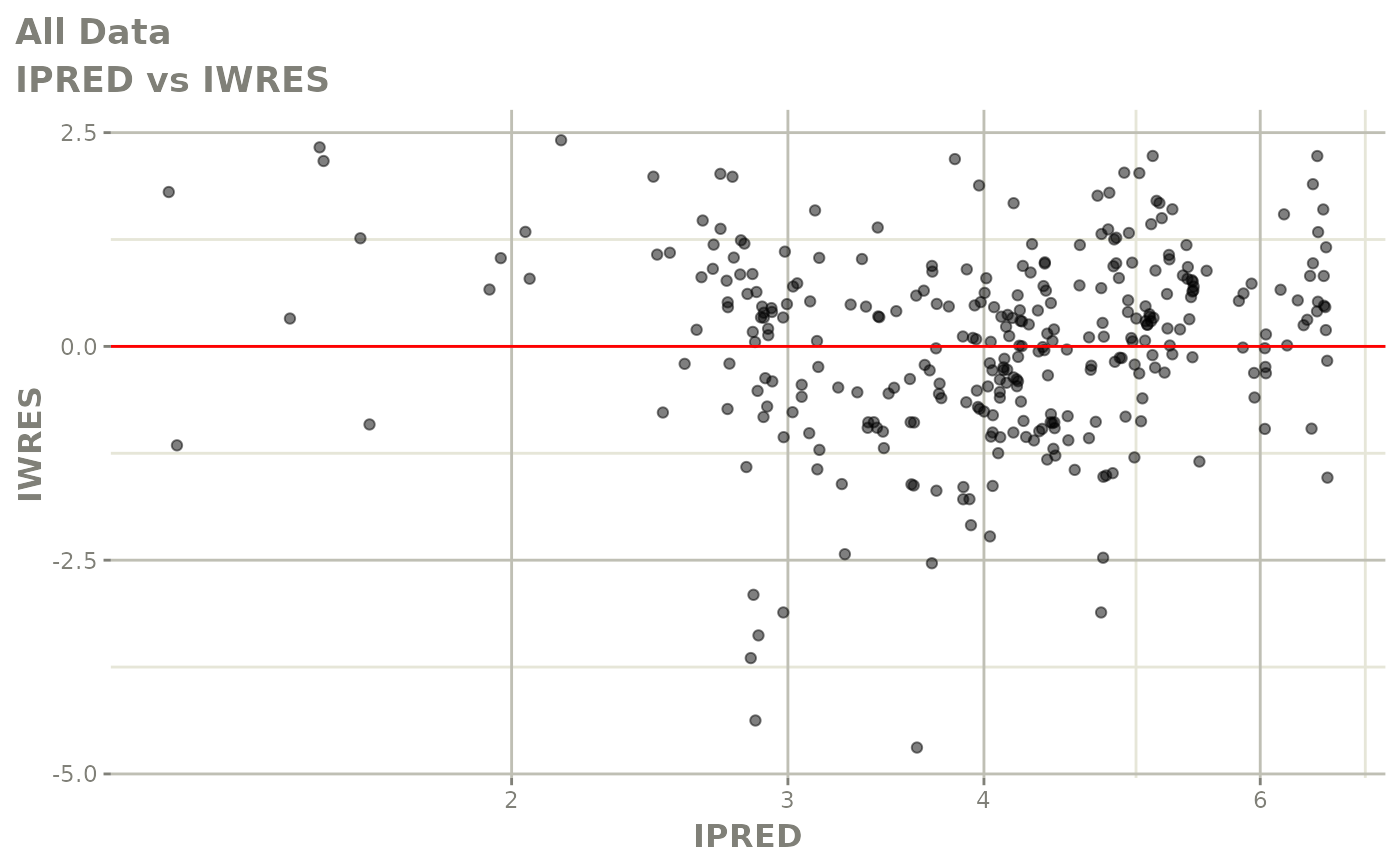
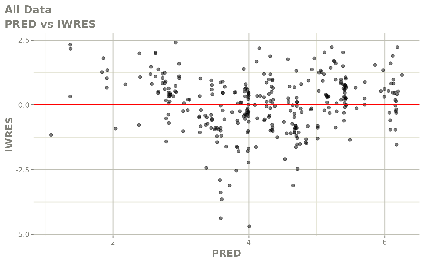
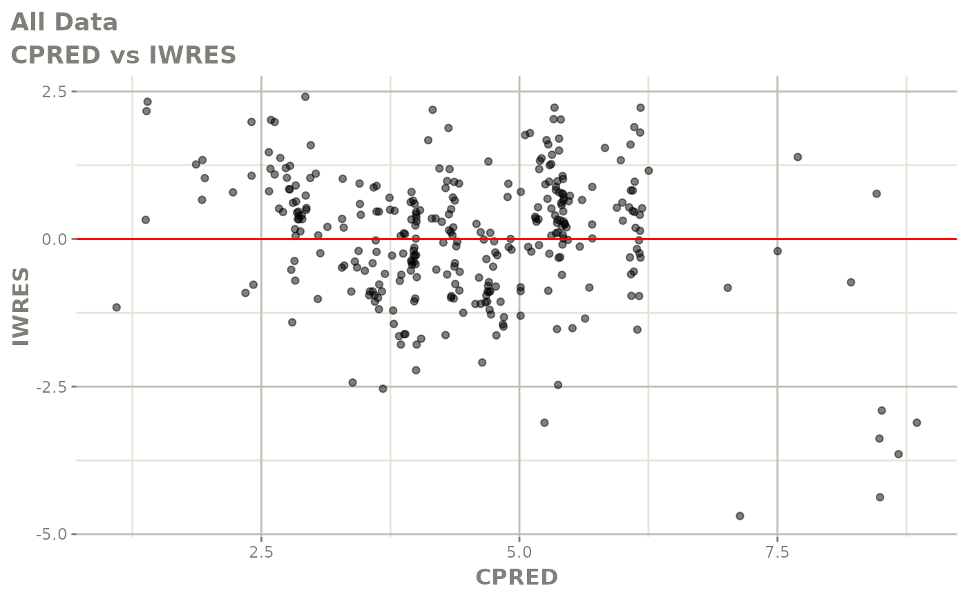
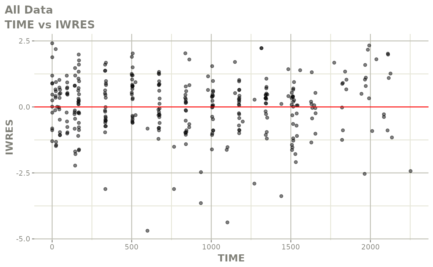
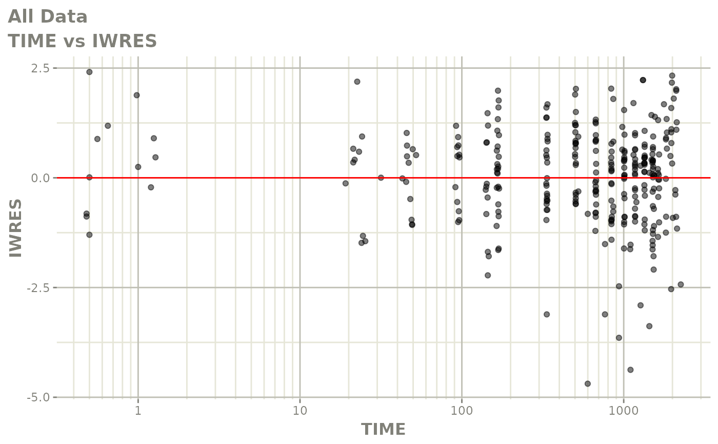
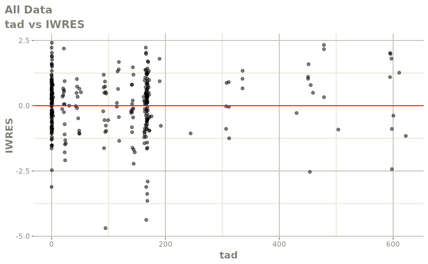
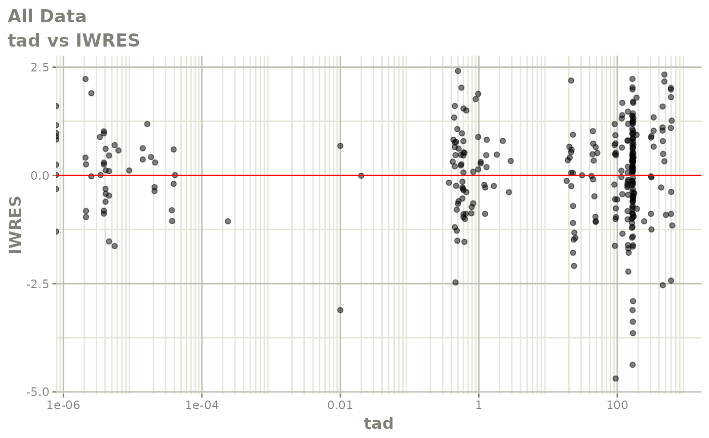
print(absval_res_vs_idv(xpdb, res = 'IWRES') +
      ylab("Individual Weighted Residuals") +
      xlab("Time (h)"))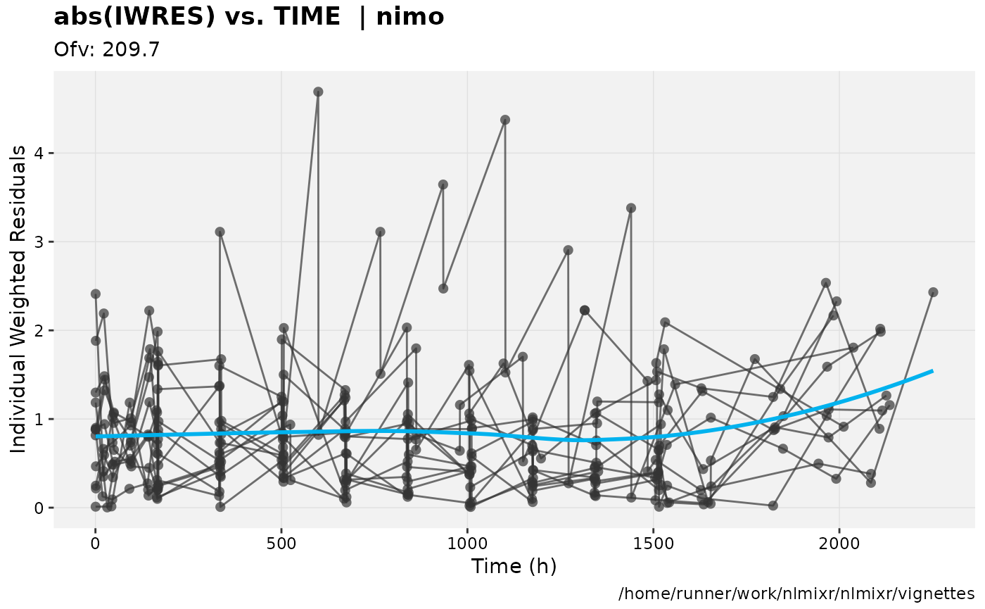

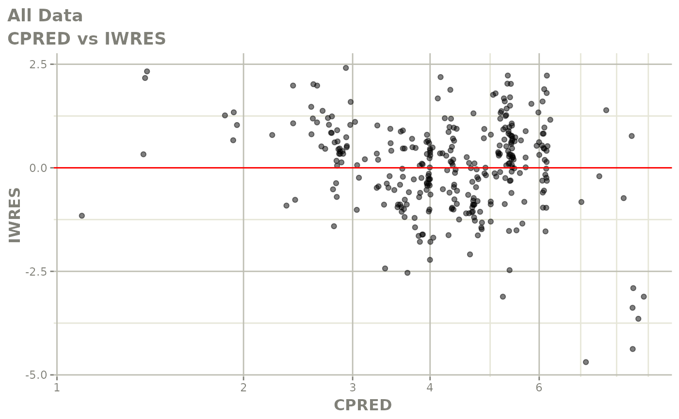
print(absval_res_vs_pred(xpdb, res = 'IWRES') +
      ylab("Individual Weighted Residuals") +
      xlab("Population Predicted Nimotuzumab Concentrations (ug/mL)"))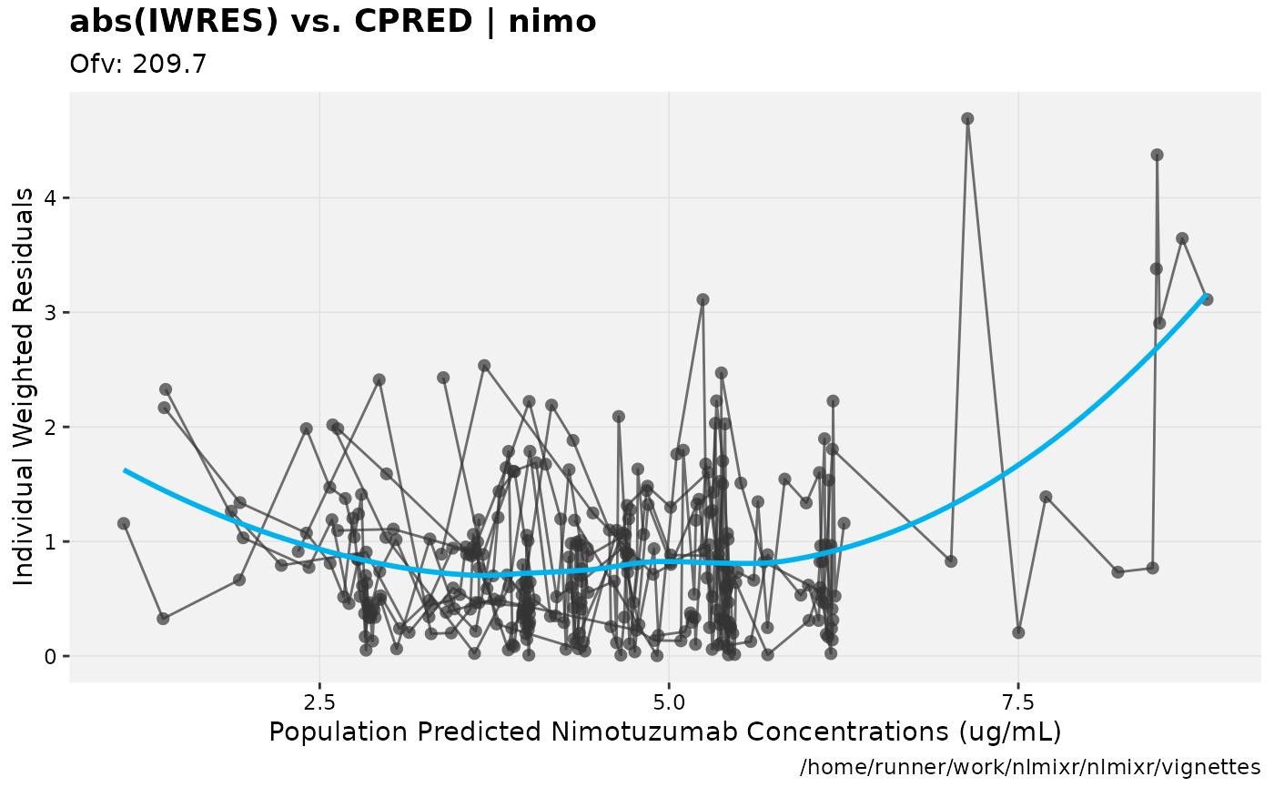

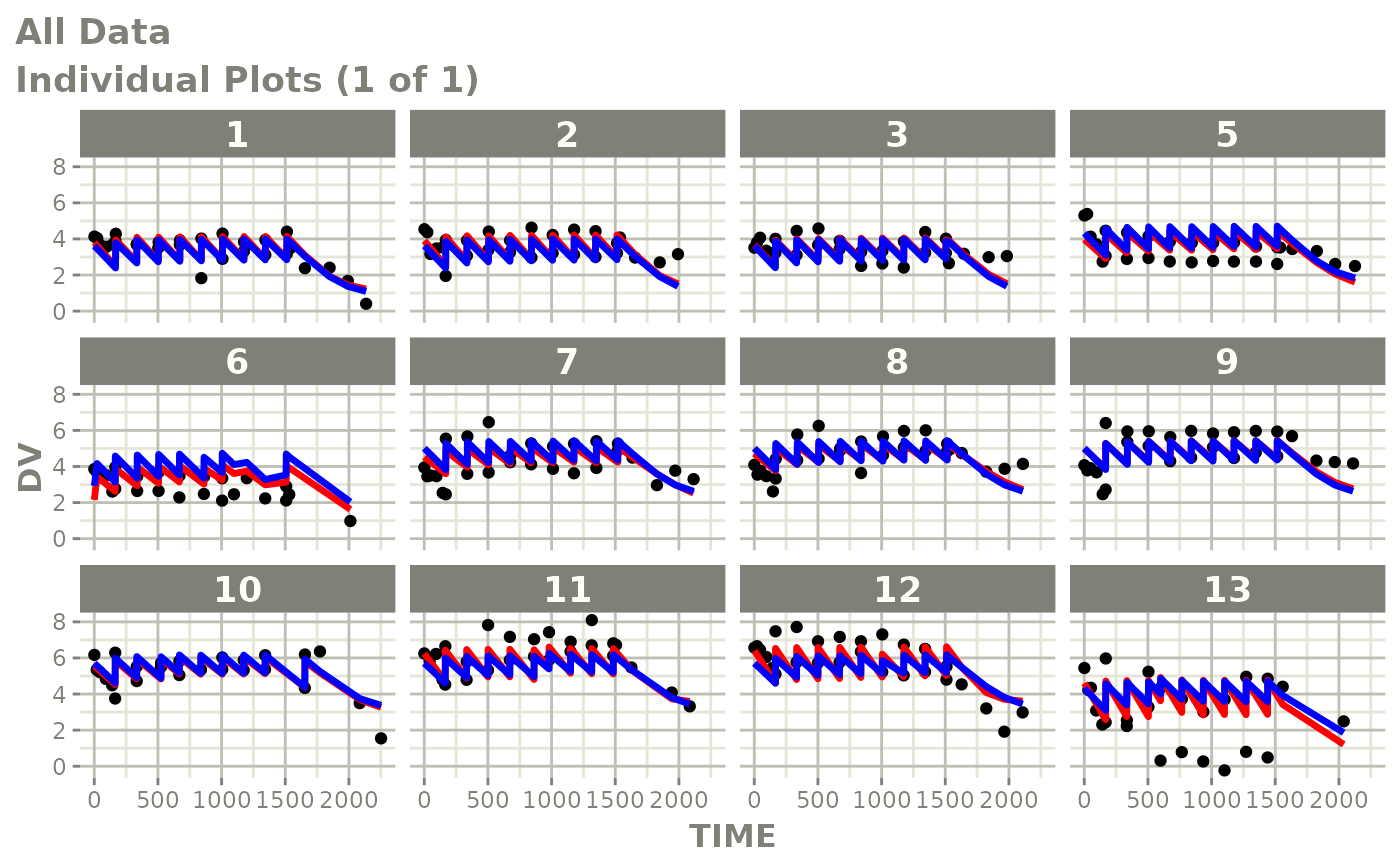
print(ind_plots(xpdb, nrow=3, ncol=4) +
      ylab("Predicted and Observed Nimotuzumab concentrations (ug/mL)") +
      xlab("Time (h)"))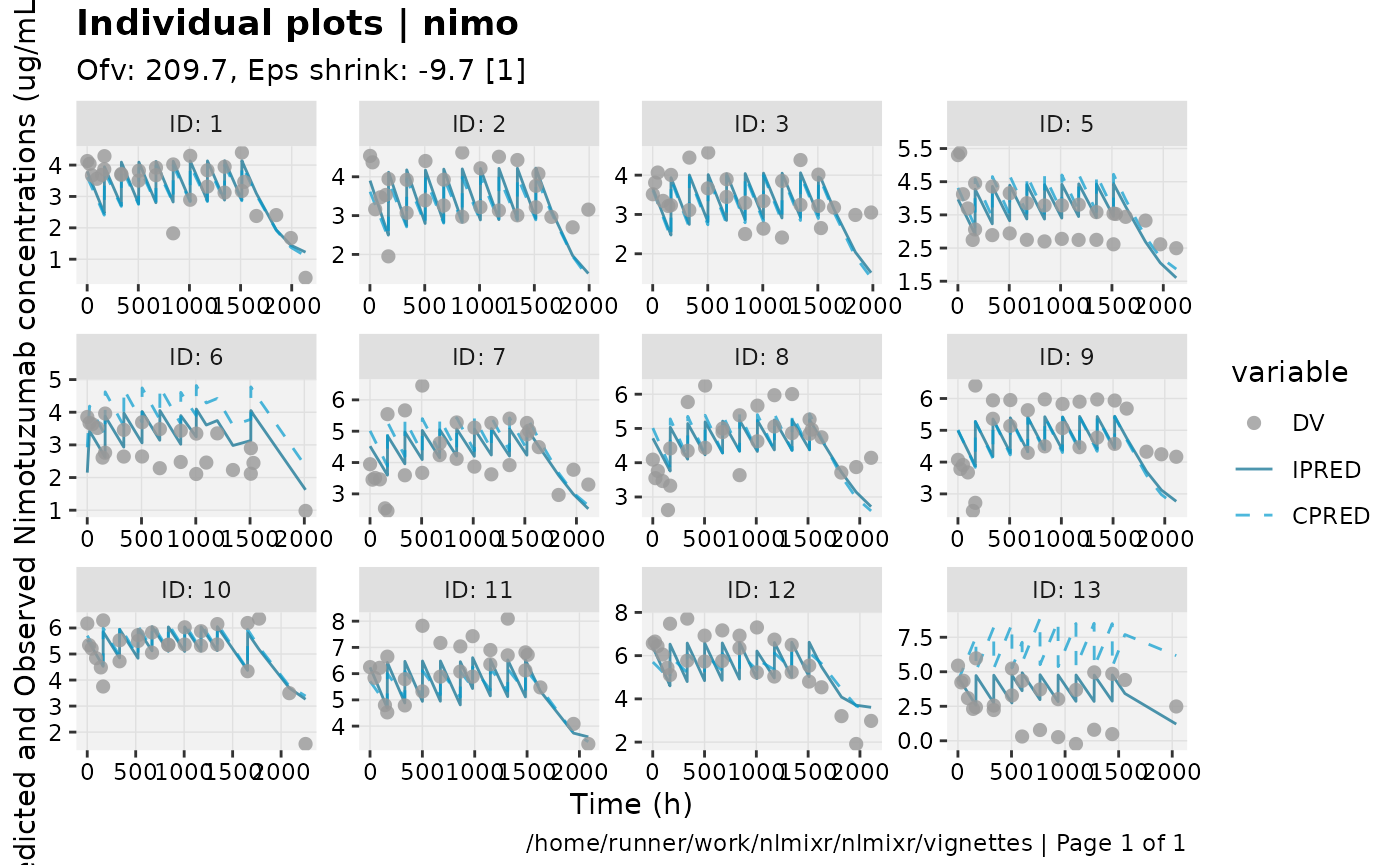

print(res_distrib(xpdb) +
     ylab("Density") +
     xlab("Conditional Weighted Residuals"))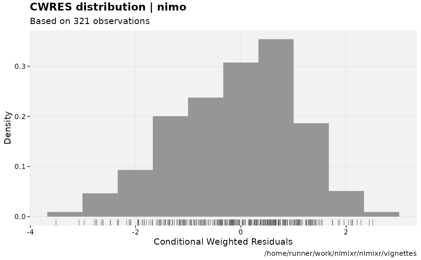

################################################################################
##Visual Predictive Checks
################################################################################
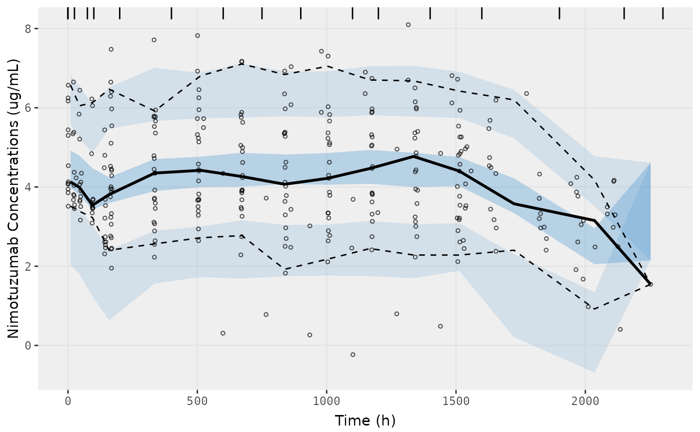
vpc.ui(fit,n=500,stratify=c("dos"), show=list(obs_dv=T),
       bins = c(-0.5,0,25,75,100,200,400,600,750,900,1100,1200,1400,1600,1900,2150,2300),
       ylab = "Nimotuzumab Concentrations (ug/mL)", xlab = "Time (h)")
#>   $rxsim = original simulated data
#>   $sim = merge simulated data
#>   $obs = observed data
#>   $gg = vpc ggplot
#> use vpc(...) to change plot options
#> plotting the object now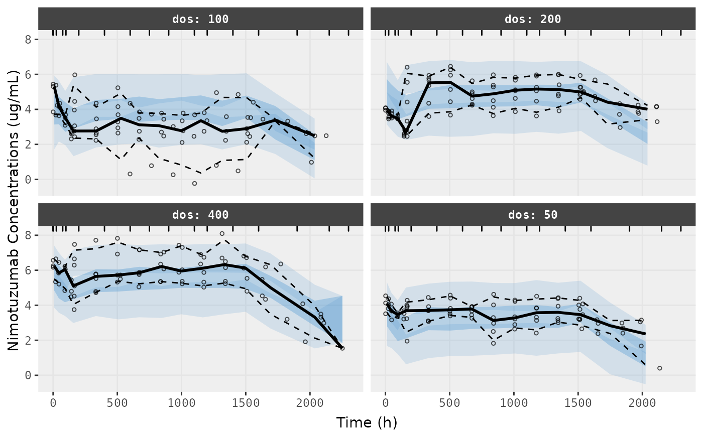

vpc.ui(fit,n=500, show=list(obs_dv=T),
       bins = c(-0.5,0,25,75,100,200,400,600,750,900,1100,1200,1400,1600,1900,2150,2300),
       ylab = "Nimotuzumab Concentrations (ug/mL)", xlab = "Time (h)")
#>   $rxsim = original simulated data
#>   $sim = merge simulated data
#>   $obs = observed data
#>   $gg = vpc ggplot
#> use vpc(...) to change plot options
#> plotting the object now