Single Subject ODE solving – differences from multiple subject
rxode-single-subject.Rmdlibrary(RxODE)Single Subject solving
Originally, RxODE was only created to solve ODEs for one individual. That is a single system without any changes in individual parameters.
Of course this is still supported, the classic examples are found in RxODE intro.
This article discusses the differences between multiple subject and single subject solving. There are three differences:
- Single solving does not solve each ID in parallel
- Single solving lacks the
idcolumn in parameters($params) as well as in the actual dataset. - Single solving allows parameter exploration easier because each parameter can be modified. With multiple subject solves, you have to make sure to update each individual parameter.
The first obvious difference is in speed; With multiple subjects you can run each subject ID in parallel. For more information and examples of the speed gains with multiple subject solving see the Speeding up RxODE vignette.
The next difference is the amount of information output in the final data.
Taking the 2 compartment indirect response model originally in the tutorial:
mod1 <-RxODE({
    KA=2.94E-01;
    CL=1.86E+01;
    V2=4.02E+01;
    Q=1.05E+01;
    V3=2.97E+02;
    Kin=1;
    Kout=1;
    EC50=200;
    C2 = centr/V2;
    C3 = peri/V3;
    d/dt(depot) =-KA*depot;
    d/dt(centr) = KA*depot - CL*C2 - Q*C2 + Q*C3;
    d/dt(peri)  =                    Q*C2 - Q*C3;
    d/dt(eff)  = Kin - Kout*(1-C2/(EC50+C2))*eff;
    eff(0) = 1
});

et <- et(amount.units='mg', time.units='hours') %>%
    et(dose=10000, addl=9, ii=12) %>%
    et(amt=20000, nbr.doses=5, start.time=120, dosing.interval=24) %>%
    et(0:240) # sampling
Now a simple solve
x <- rxSolve(mod1, et)
x
#> ▂▂▂▂▂▂▂▂▂▂▂▂▂▂▂▂▂▂▂▂▂▂▂▂▂▂▂ Solved RxODE object ▂▂▂▂▂▂▂▂▂▂▂▂▂▂▂▂▂▂▂▂▂▂▂▂▂▂▂
#> ── Parameters (x$params): ─────────────────────────────────────────────────
#>
#>      KA      CL      V2       Q      V3     Kin    Kout    EC50
#>   0.294  18.600  40.200  10.500 297.000   1.000   1.000 200.000
#> ── Initial Conditions (x$inits): ──────────────────────────────────────────
#> depot centr  peri   eff
#>     0     0     0     1
#> ── First part of data (object): ───────────────────────────────────────────
#> # A tibble: 241 x 7
#>    time    C2    C3  depot centr  peri   eff
#>     [h] <dbl> <dbl>  <dbl> <dbl> <dbl> <dbl>
#> 1     0   0   0     10000     0     0   1
#> 2     1  44.4 0.920  7453. 1784.  273.  1.08
#> 3     2  54.9 2.67   5554. 2206.  794.  1.18
#> 4     3  51.9 4.46   4140. 2087. 1324.  1.23
#> 5     4  44.5 5.98   3085. 1789. 1776.  1.23
#> 6     5  36.5 7.18   2299. 1467. 2132.  1.21
#> # … with 235 more rows
#> ▂▂▂▂▂▂▂▂▂▂▂▂▂▂▂▂▂▂▂▂▂▂▂▂▂▂▂▂▂▂▂▂▂▂▂▂▂▂▂▂▂▂▂▂▂▂▂▂▂▂▂▂▂▂▂▂▂▂▂▂▂▂▂▂▂▂▂▂▂▂▂▂▂▂▂

print(x)
#> ▂▂▂▂▂▂▂▂▂▂▂▂▂▂▂▂▂▂▂▂▂▂▂▂▂▂▂ Solved RxODE object ▂▂▂▂▂▂▂▂▂▂▂▂▂▂▂▂▂▂▂▂▂▂▂▂▂▂▂
#> ── Parameters ($params): ──────────────────────────────────────────────────
#>
#>      KA      CL      V2       Q      V3     Kin    Kout    EC50
#>   0.294  18.600  40.200  10.500 297.000   1.000   1.000 200.000
#> ── Initial Conditions ($inits): ───────────────────────────────────────────
#> depot centr  peri   eff
#>     0     0     0     1
#> ── First part of data (object): ───────────────────────────────────────────
#> # A tibble: 241 x 7
#>    time    C2    C3  depot centr  peri   eff
#>     [h] <dbl> <dbl>  <dbl> <dbl> <dbl> <dbl>
#> 1     0   0   0     10000     0     0   1
#> 2     1  44.4 0.920  7453. 1784.  273.  1.08
#> 3     2  54.9 2.67   5554. 2206.  794.  1.18
#> 4     3  51.9 4.46   4140. 2087. 1324.  1.23
#> 5     4  44.5 5.98   3085. 1789. 1776.  1.23
#> 6     5  36.5 7.18   2299. 1467. 2132.  1.21
#> # … with 235 more rows
#> ▂▂▂▂▂▂▂▂▂▂▂▂▂▂▂▂▂▂▂▂▂▂▂▂▂▂▂▂▂▂▂▂▂▂▂▂▂▂▂▂▂▂▂▂▂▂▂▂▂▂▂▂▂▂▂▂▂▂▂▂▂▂▂▂▂▂▂▂▂▂▂▂▂▂▂

plot(x, C2, eff)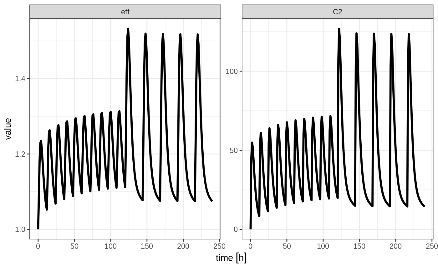
To better see the differences between the single solve, you can solve for 2 individuals
x2 <- rxSolve(mod1, et %>% et(id=1:2), params=data.frame(CL=c(18.6, 7.6)))
#> Warning in (function (idData, goodLvl, type = "parameter", warnIdSort) : ID missing in parameters dataset;
#>  Parameters are assumed to have the same order as the IDs in the event dataset
print(x2)
#> ▂▂▂▂▂▂▂▂▂▂▂▂▂▂▂▂▂▂▂▂▂▂▂▂▂▂▂ Solved RxODE object ▂▂▂▂▂▂▂▂▂▂▂▂▂▂▂▂▂▂▂▂▂▂▂▂▂▂▂
#> ── Initial Conditions ($inits): ───────────────────────────────────────────
#> depot centr  peri   eff
#>     0     0     0     1
#> ── First part of data (object): ───────────────────────────────────────────
#> # A tibble: 482 x 8
#>   id     time    C2    C3  depot centr  peri   eff
#>   <fct>   [h] <dbl> <dbl>  <dbl> <dbl> <dbl> <dbl>
#> 1 1         0   0   0     10000     0     0   1
#> 2 1         1  44.4 0.920  7453. 1784.  273.  1.08
#> 3 1         2  54.9 2.67   5554. 2206.  794.  1.18
#> 4 1         3  51.9 4.46   4140. 2087. 1324.  1.23
#> 5 1         4  44.5 5.98   3085. 1789. 1776.  1.23
#> 6 1         5  36.5 7.18   2299. 1467. 2132.  1.21
#> # … with 476 more rows
#> ▂▂▂▂▂▂▂▂▂▂▂▂▂▂▂▂▂▂▂▂▂▂▂▂▂▂▂▂▂▂▂▂▂▂▂▂▂▂▂▂▂▂▂▂▂▂▂▂▂▂▂▂▂▂▂▂▂▂▂▂▂▂▂▂▂▂▂▂▂▂▂▂▂▂▂

plot(x2, C2, eff)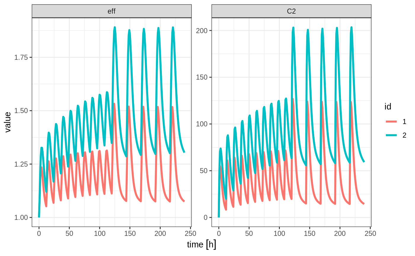
By observing the two solves, you can see:
- A multiple subject solve contains the
idcolumn both in the data frame and then data frame of parameters for each subject.
The last feature that is not as obvious, modifying the individual parameters. For single subject data, you can modify the RxODE data frame changing initial conditions and parameter values as if they were part of the data frame, as described in the RxODE Data Frames.
For multiple subject solving, this feature still works, but requires care when supplying each individual’s parameter value, otherwise you may change the solve and drop parameter for key individuals.
Summary of Single solve vs Multiple subject solving
| Feature | Single Subject Solve | Multiple Subject Solve |
|---|---|---|
| Parallel | None | Each Subject |
| $params | data.frame with one parameter value | data.frame with one parameter per subject (w/ID column) |
| solved data | Can modify individual parameters with $ syntax | Have to modify all the parameters to update solved object |
Session Information
The session information:
sessionInfo()
#> R version 3.6.0 (2019-04-26)
#> Platform: x86_64-pc-linux-gnu (64-bit)
#> Running under: Gentoo/Linux
#>
#> Matrix products: default
#> BLAS:   /usr/lib64/libblas.so.3.8.0
#> LAPACK: /usr/lib64/liblapack.so.3.8.0
#>
#> locale:
#>  [1] LC_CTYPE=en_US.utf8       LC_NUMERIC=C
#>  [3] LC_TIME=en_US.utf8        LC_COLLATE=en_US.utf8
#>  [5] LC_MONETARY=en_US.utf8    LC_MESSAGES=en_US.utf8
#>  [7] LC_PAPER=en_US.utf8       LC_NAME=C
#>  [9] LC_ADDRESS=C              LC_TELEPHONE=C
#> [11] LC_MEASUREMENT=en_US.utf8 LC_IDENTIFICATION=C
#>
#> attached base packages:
#> [1] stats     graphics  grDevices utils     datasets  methods   base
#>
#> other attached packages:
#> [1] RxODE_0.9.1-7
#>
#> loaded via a namespace (and not attached):
#>  [1] Rcpp_1.0.2       compiler_3.6.0   pillar_1.4.2     sys_3.3
#>  [5] PreciseSums_0.3  tools_3.6.0      zeallot_0.1.0    mvnfast_0.2.5
#>  [9] digest_0.6.21    evaluate_0.14    memoise_1.1.0    tibble_2.1.3
#> [13] gtable_0.3.0     pkgconfig_2.0.3  rlang_0.4.0      cli_1.1.0
#> [17] yaml_2.2.0       pkgdown_1.4.1    xfun_0.10        stringr_1.4.0
#> [21] dplyr_0.8.3      knitr_1.25       vctrs_0.2.0      desc_1.2.0
#> [25] fs_1.3.1         rprojroot_1.3-2  grid_3.6.0       tidyselect_0.2.5
#> [29] glue_1.3.1       R6_2.4.0         fansi_0.4.0      rmarkdown_1.16
#> [33] polyclip_1.10-0  dparser_1.3.1-0  farver_1.1.0     ggplot2_3.2.1
#> [37] purrr_0.3.2      tweenr_1.0.1     magrittr_1.5     units_0.6-5
#> [41] backports_1.1.5  scales_1.0.0     htmltools_0.4.0  MASS_7.3-51.4
#> [45] assertthat_0.2.1 ggforce_0.3.1    colorspace_1.4-1 labeling_0.3
#> [49] utf8_1.1.4       lotri_0.1.1      stringi_1.4.3    lazyeval_0.2.2
#> [53] munsell_0.5.0    crayon_1.3.4