RxODE Simulation
2019-10-16
RxODE-sim-var.Rmd
Population Simulations with RxODE
Simulation of Variability with RxODE
In pharmacometrics the nonlinear-mixed effect modeling software (like nlmixr) characterizes the between-subject variability. With this between subject variability you can simulate new subjects.
Assuming that you have a 2-compartment, indirect response model, you can set create an RxODE model describing this system below:
Adding the parameter estimates
The next step is to get the parameters into R so that you can start the simulation:
theta <- c(KA=2.94E-01, TCl=1.86E+01, V2=4.02E+01,  # central
           Q=1.05E+01, V3=2.97E+02,                # peripheral
           Kin=1, Kout=1, EC50=200, prop.err=0)      # effects
In this case, I use lotri to specify the omega since it uses similar lower-triangular matrix specification as nlmixr (also similar to NONMEM):
## the column names of the omega matrix need to match the parameters specified by RxODE
omega <- lotri(eta.Cl ~ 0.4^2)
omega
#>        eta.Cl
#> eta.Cl   0.16
Simulating
The next step to simulate is to create the dosing regimen for overall simulation:
If you wish, you can also add sampling times (though now RxODE can fill these in for you):
ev <- ev %>% et(0,48, length.out=100);Note the et takes similar arguments as seq when adding sampling times. There are more methods to adding sampling times and events to make complex dosing regimens (See the event vignette). This includes ways to add variability to the both the sampling and dosing times).
Once this is complete you can simulate using the rxSolve routine:
sim <- rxSolve(mod,theta,ev,omega=omega,nSub=100)To quickly look and customize your simulation you use the default plot routine. Since this is an RxODE object, it will create a ggplot2 object that you can modify as you wish. The extra parameter to the plot tells RxODE/R what piece of information you are interested in plotting. In this case, we are interested in looking at the derived parameter C2:
Checking the simulation by a simple ggplot
library(ggplot2)

plot(sim, C2) +
    coord_trans(y = "log10") +
    ylab("Central Compartment") +
    xlab("Time") +
    guides(color=FALSE)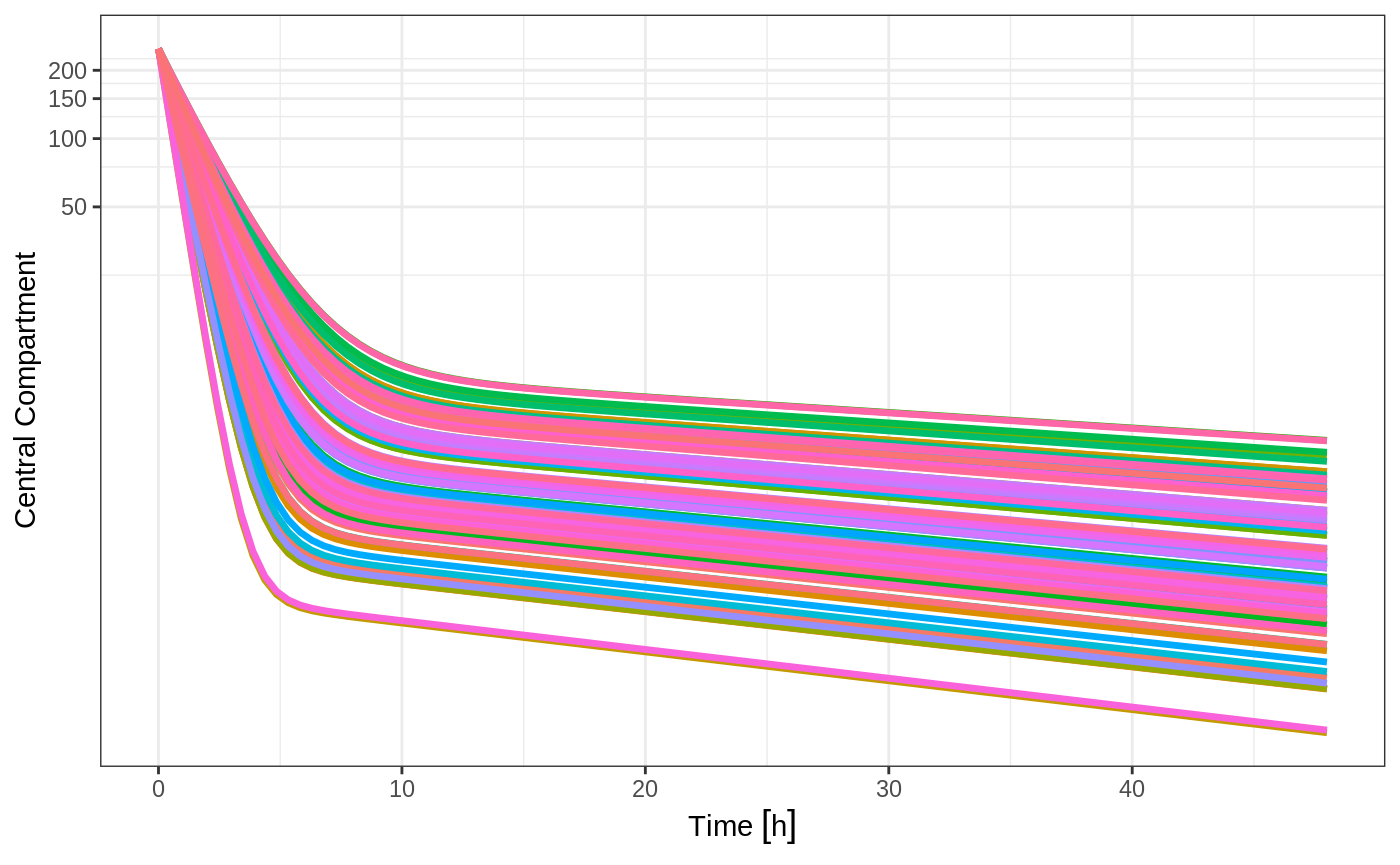
Of course this additional parameter could also be a state value, like eff:
plot(sim, "eff") +
    coord_trans(y = "log10") +
    ylab("Effect") +
    xlab("Time") +
    guides(color=FALSE)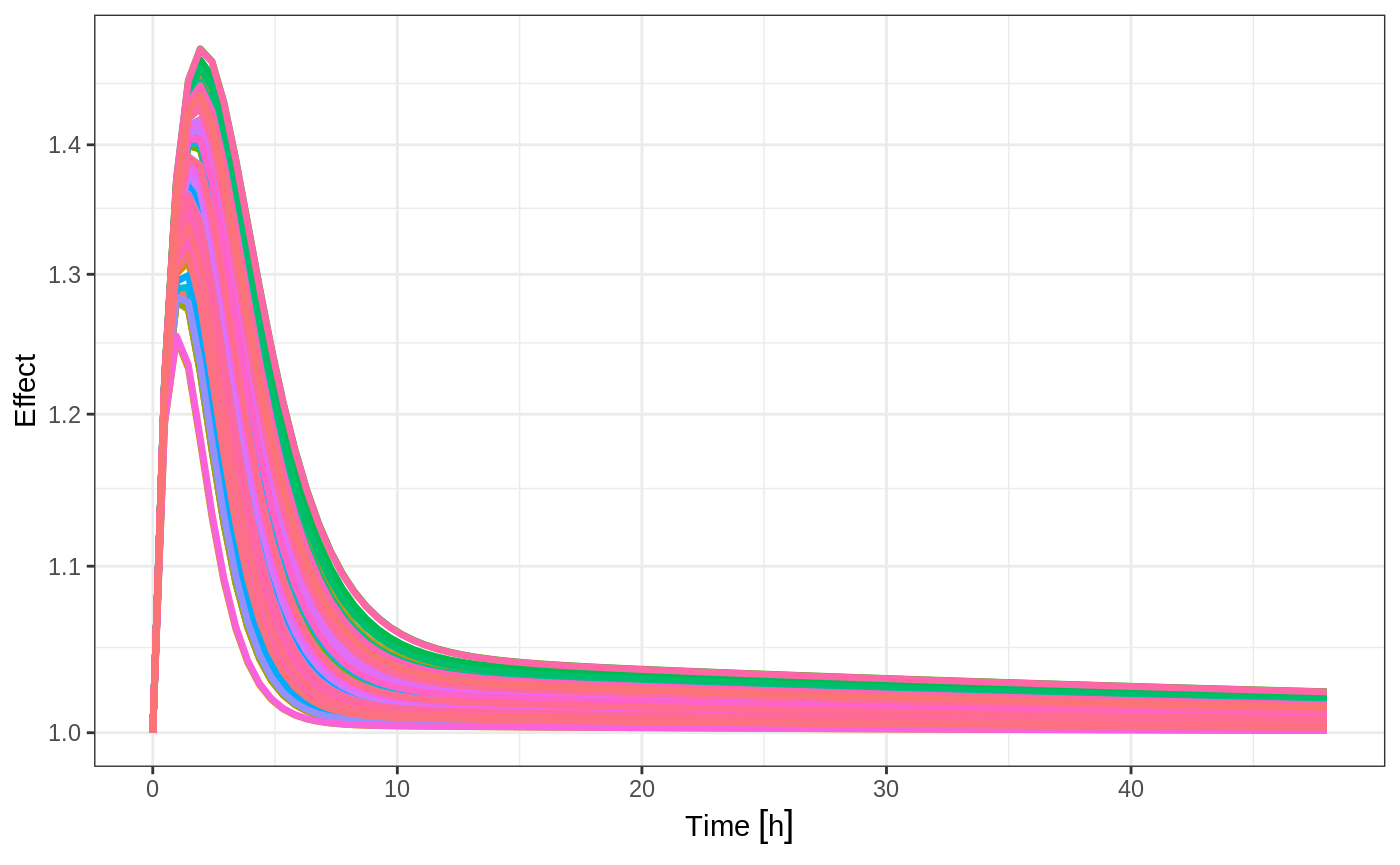
Or you could even look at the two side-by-side:
plot(sim, C2, eff) +
    coord_trans(y = "log10") +
    ylab("Effect") +
    xlab("Time") +
    guides(color=FALSE)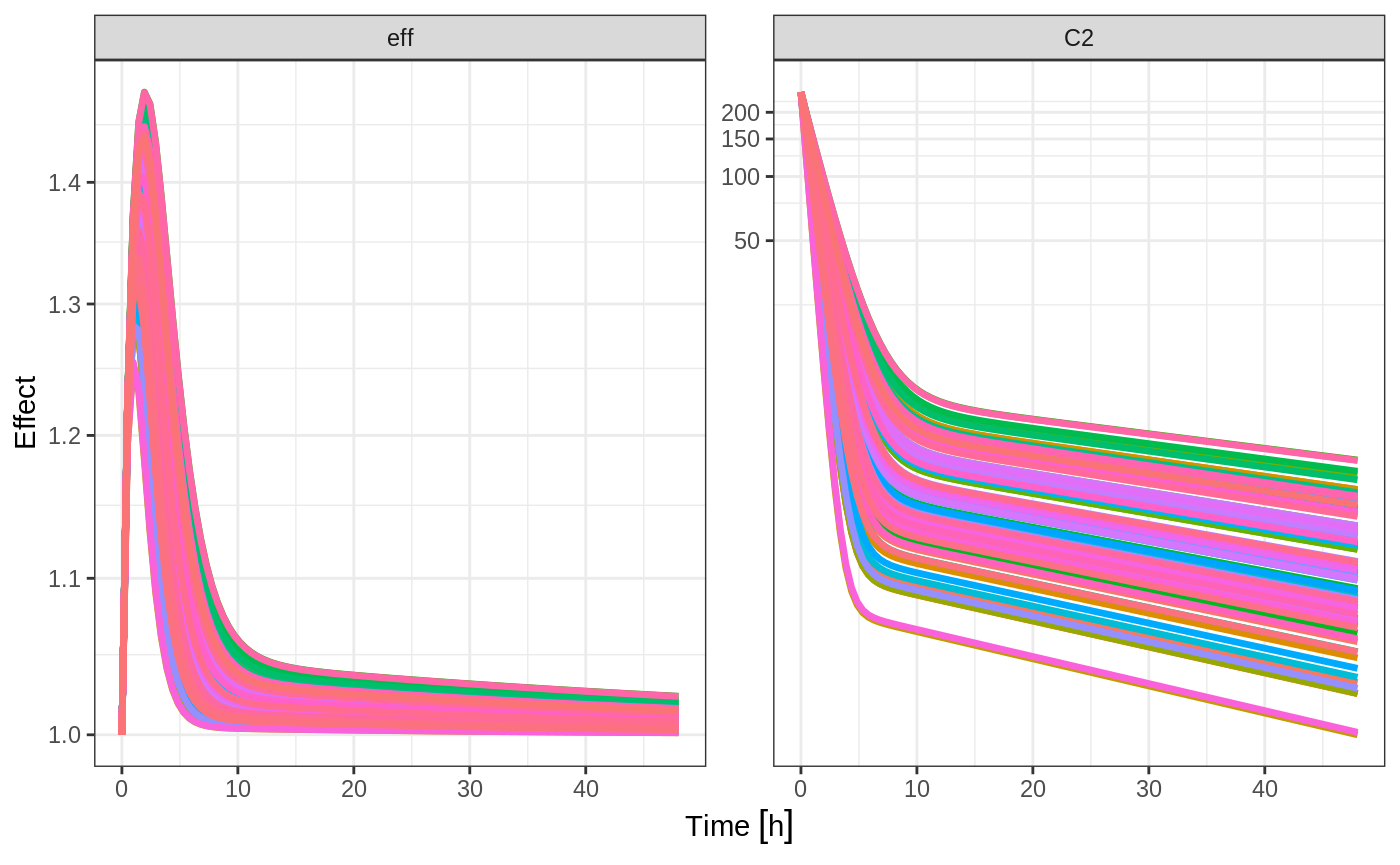
Processing the data to create summary plots
Usually in pharmacometric simulations it is not enough to simply simulate the system. We have to do something easier to digest, like look at the central and extreme tendencies of the simulation.
Since the RxODE solve object is a type of data frame
It is now straightforward to perform calculations and generate plots with the simulated data. Below, the 5th, 50th, and 95th percentiles of the simulated data are plotted.
library(dplyr)
#>
#> Attaching package: 'dplyr'
#> The following objects are masked from 'package:stats':
#>
#>     filter, lag
#> The following objects are masked from 'package:base':
#>
#>     intersect, setdiff, setequal, union
library(ggplot2)

p <- c(0.05, 0.5, 0.95);
s <-sim %>% group_by(time) %>%
    do(data.frame(p=p, eff=quantile(.$eff, probs=p),
                  eff.n = length(.$eff), eff.avg = mean(.$eff),
                  centr=quantile(.$centr, probs=p),
                  centr.n=length(.$centr),centr.avg = mean(.$centr))) %>%
    mutate(Percentile=factor(sprintf("%d%%",p*100),levels=c("5%","50%","95%")))

ggplot(s,aes(time,centr,color=Percentile)) + geom_line(size=1) + coord_trans(y = "log10") + ylab("Central Concentration") +
    xlab("Time")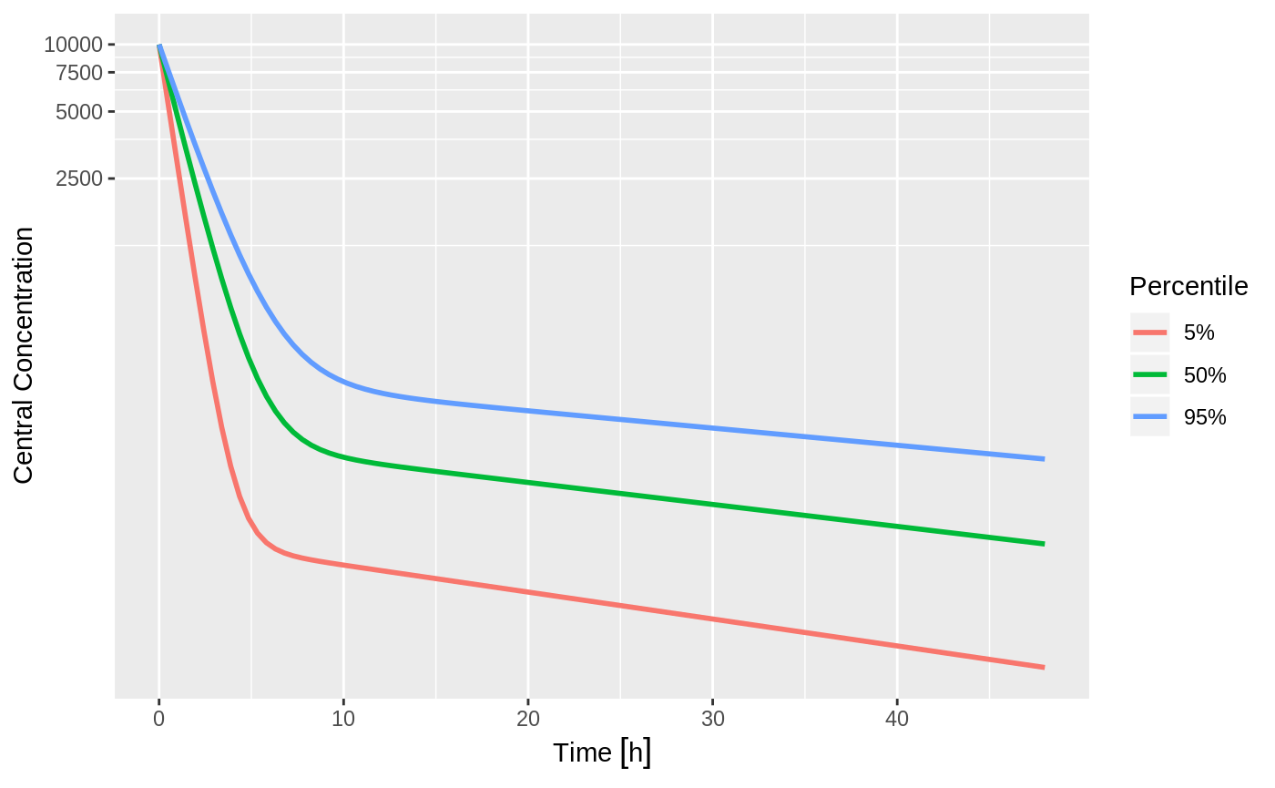
ggplot(s,aes(time,eff,color=Percentile)) + geom_line(size=1) + ylab("Effect") +
    xlab("Time") + guides(color=FALSE)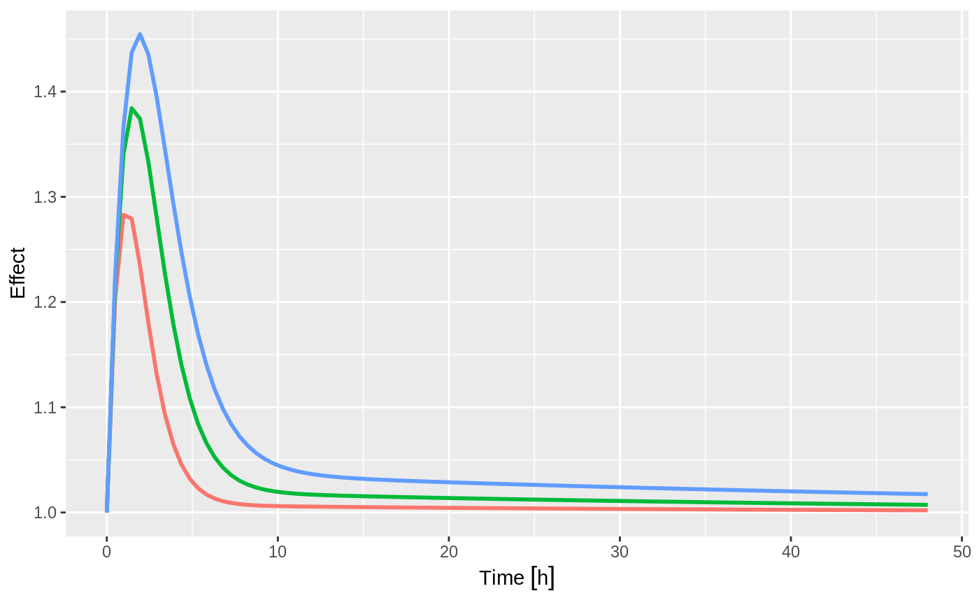
Note that you can see the parameters that were simulated for the example
head(sim$param)
#>   sim.id   V2 prop.err  V3  TCl     eta.Cl    KA    Q Kin Kout EC50
#> 1      1 40.2        0 297 18.6 0.49671545 0.294 10.5   1    1  200
#> 2      2 40.2        0 297 18.6 0.73373376 0.294 10.5   1    1  200
#> 3      3 40.2        0 297 18.6 0.01268888 0.294 10.5   1    1  200
#> 4      4 40.2        0 297 18.6 0.79537016 0.294 10.5   1    1  200
#> 5      5 40.2        0 297 18.6 0.07905109 0.294 10.5   1    1  200
#> 6      6 40.2        0 297 18.6 0.79755744 0.294 10.5   1    1  200
Simulation of unexplained variability
In addition to conveniently simulating between subject variability, you can also easily simulate unexplained variability.
mod <- RxODE({
    eff(0) = 1
    C2 = centr/V2;
    C3 = peri/V3;
    CL =  TCl*exp(eta.Cl) ## This is coded as a variable in the model
    d/dt(depot) =-KA*depot;
    d/dt(centr) = KA*depot - CL*C2 - Q*C2 + Q*C3;
    d/dt(peri)  =                    Q*C2 - Q*C3;
    d/dt(eff)  = Kin - Kout*(1-C2/(EC50+C2))*eff;
    e = eff+eff.err
    cp = centr*(1+cp.err)
})

theta <- c(KA=2.94E-01, TCl=1.86E+01, V2=4.02E+01,  # central
           Q=1.05E+01, V3=2.97E+02,                # peripheral
           Kin=1, Kout=1, EC50=200)                # effects

sigma <- lotri(eff.err ~ 0.1, cp.err ~ 0.1)


sim  <- rxSolve(mod, theta, ev, omega=omega, nSub=100, sigma=sigma)
s <- confint(sim, c("eff", "centr"));
#> Warning in confint.rxSolve(sim, c("eff", "centr")): In order to put
#> confidence bands around the intervals, you need at least 2500 simulations.
#> Summarizing data
#> done.

plot(s)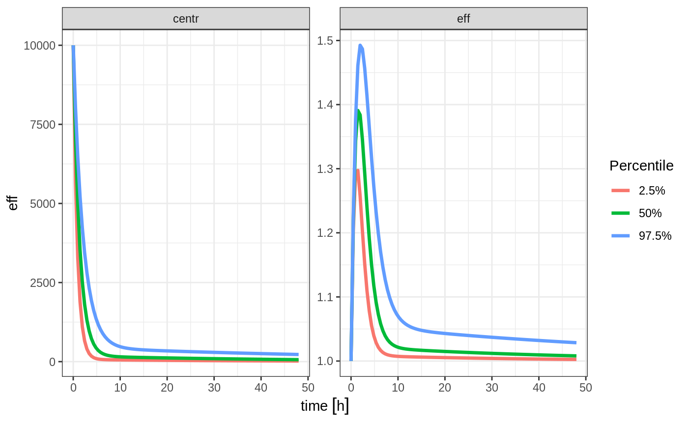
Simulation of Individuals
Sometimes you may want to match the dosing and observations of individuals in a clinical trial. To do this you will have to create a data.frame using the RxODE event specification as well as an ID column to indicate an individual. The RxODE event vignette talks more about how these datasets should be created.
ev1 <- eventTable(amount.units="mg", time.units="hours") %>%
    add.dosing(dose=10000, nbr.doses=1, dosing.to=2) %>%
    add.sampling(seq(0,48,length.out=10));

ev2 <- eventTable(amount.units="mg", time.units="hours") %>%
    add.dosing(dose=5000, nbr.doses=1, dosing.to=2) %>%
    add.sampling(seq(0,48,length.out=8));

dat <- rbind(data.frame(ID=1, ev1$get.EventTable()),
             data.frame(ID=2, ev2$get.EventTable()))


## Note the number of subject is not needed since it is determined by the data
sim  <- rxSolve(mod, theta, dat, omega=omega, sigma=sigma)
#> Warning in (function (idData, goodLvl, type = "parameter", warnIdSort) : ID missing in parameters dataset;
#>  Parameters are assumed to have the same order as the IDs in the event dataset

sim %>% select(id, time, e, cp)
#>    id          time         e         cp
#> 1   1  0.000000 [h] 0.8260474 7882.44548
#> 2   1  5.333333 [h] 1.4578039  820.25185
#> 3   1 10.666667 [h] 0.7906930  336.60578
#> 4   1 16.000000 [h] 1.2523168  276.03724
#> 5   1 21.333333 [h] 0.4408824  142.13458
#> 6   1 26.666667 [h] 1.8284991  113.99939
#> 7   1 32.000000 [h] 1.2463638  169.19089
#> 8   1 37.333333 [h] 0.6831690  165.04934
#> 9   1 42.666667 [h] 1.1548495   51.12333
#> 10  1 48.000000 [h] 0.4831699   76.18043
#> 11  2  0.000000 [h] 0.5909889 1565.32313
#> 12  2  6.857143 [h] 0.6781570  115.66227
#> 13  2 13.714286 [h] 0.8340606  121.88295
#> 14  2 20.571429 [h] 0.9249224   91.32832
#> 15  2 27.428571 [h] 0.3134112   46.35293
#> 16  2 34.285714 [h] 0.6307752   67.28990
#> 17  2 41.142857 [h] 1.0858981   36.09942
#> 18  2 48.000000 [h] 0.6637714   26.48440
Simulation of Clinical Trials
By either using a simple single event table, or data from a clinical trial as described above, a complete clinical trial simulation can be performed.
Typically in clinical trial simulations you want to account for the uncertainty in the fixed parameter estimates, and even the uncertainty in both your between subject variability as well as the unexplained variability.
RxODE allows you to account for these uncertainties by simulating multiple virtual “studies,” specified by the parameter nStud. In a single virtual study:
A Population effect parameter is sampled from a multivariate normal distribution with mean given by the parameter estimates and the variance specified by the named matrix
thetaMat.A between subject variability/covariance matrix is sampled from either a scaled inverse chi-squared distribution (for the univariate case) or a inverse Wishart that is parameterized to scale to the conjugate prior covariance term, as described by the wikipedia article. (This is not the same as the scaled inverse Wishart distribution ). In the case of the between subject variability, the variance/covariance matrix is given by the ‘omega’ matrix parameter and the degrees of freedom is the number of subjects in the simulation.
Unexplained variability is also simulated from the scaled inverse chi squared distribution or inverse Wishart distribution with the variance/covariance matrix given by the ‘sigma’ matrix parameter and the degrees of freedom given by the number of observations being simulated.
The covariance/variance prior is simulated from RxODEs cvPost() function.
An example of this simulation is below:
## Creating covariance matrix
tmp <- matrix(rnorm(8^2), 8, 8)
tMat <- tcrossprod(tmp, tmp) / (8 ^ 2)
dimnames(tMat) <- list(NULL, names(theta))

sim  <- rxSolve(mod, theta, ev, omega=omega, nSub=100, sigma=sigma, thetaMat=tMat, nStud=10,
                dfSub=10, dfObs=100)

s <-sim %>% confint(c("centr", "eff"))
#> Summarizing data
#> done.

plot(s)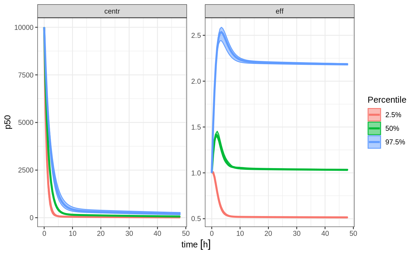
If you wish you can see what omega and sigma was used for each virtual study by accessing them in the solved data object with $omega.list and $sigma.list:
head(sim$omega.list)
#> [[1]]
#>           [,1]
#> [1,] 0.1476211
#>
#> [[2]]
#>           [,1]
#> [1,] 0.1248491
#>
#> [[3]]
#>           [,1]
#> [1,] 0.1273202
#>
#> [[4]]
#>           [,1]
#> [1,] 0.1034848
#>
#> [[5]]
#>           [,1]
#> [1,] 0.1914239
#>
#> [[6]]
#>           [,1]
#> [1,] 0.2549919head(sim$sigma.list)
#> [[1]]
#> [,1] [,2]
#> [1,] 0.10814880 0.01101639
#> [2,] 0.01101639 0.08095732
#>
#> [[2]]
#> [,1] [,2]
#> [1,] 0.07746784 0.0122470
#> [2,] 0.01224700 0.1015528
#>
#> [[3]]
#> [,1] [,2]
#> [1,] 0.1150243835 -0.0007083945
#> [2,] -0.0007083945 0.1110771033
#>
#> [[4]]
#> [,1] [,2]
#> [1,] 0.08892233 -0.01079685
#> [2,] -0.01079685 0.11192963
#>
#> [[5]]
#> [,1] [,2]
#> [1,] 0.093897270 -0.007474418
#> [2,] -0.007474418 0.113926980
#>
#> [[6]]
#> [,1] [,2]
#> [1,] 0.092846534 0.009478026
#> [2,] 0.009478026 0.121707250You can also see the parameter realizations from the $params data frame.
If you do not wish to sample from the prior distributions of either the omega or sigma matrices, you can turn off this feature by specifying the simVariability = FALSE option when solving:
sim  <- rxSolve(mod, theta, ev, omega=omega, nSub=100, sigma=sigma, thetaMat=tMat, nStud=10,
                simVariability=FALSE);

s <-sim %>% confint(c("centr", "eff"))
#> Summarizing data
#> done.

plot(s)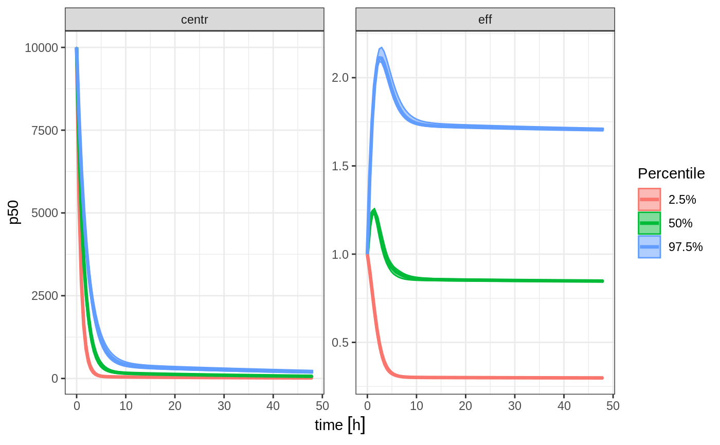
Note since realizations of omega and sigma were not simulated, $omega.list and $sigma.list both return NULL.
RxODE multi-threaded solving and simulation
RxODE now supports multi-threaded solving on OpenMP supported compilers, including linux and windows. Mac OSX can also be supported By default it uses all your available cores for solving as determined by rxCores(). This may be overkill depending on your system, at a certain point the speed of solving is limited by things other than computing power.
You can also speed up simulation by using the multi-cores to generate random deviates with mvnfast (either mvnfast::rmvn() or mvnfast::rmvt()). This is controlled by the nCoresRV parameter. For example:
sim  <- rxSolve(mod, theta, ev, omega=omega, nSub=100, sigma=sigma, thetaMat=tMat, nStud=10,
                nCoresRV=2);

p <- c(0.05, 0.5, 0.95);
s <-sim %>% confint(c("eff", "centr"))
#> Summarizing data
#> done.
The default for this is 1 core since the result depends on the number of cores and the random seed you use in your simulation. However, you can always speed up this process with more cores if you are sure your collaborators have the same number of cores available to them and have OpenMP thread-capable compile.