RxODE Data Frames
2019-10-16
RxODE-data-frame.Rmd
```
Using RxODE data frames
Creating an interactive data frame
RxODE supports returning a solved object that is a modified data-frame. This is done by the predict(), solve(), or rxSolve() methods.
library(RxODE)
library(units)

## Setup example model
mod1 <-RxODE({
    C2 = centr/V2;
    C3 = peri/V3;
    d/dt(depot) =-KA*depot;
    d/dt(centr) = KA*depot - CL*C2 - Q*C2 + Q*C3;
    d/dt(peri)  =                    Q*C2 - Q*C3;
    d/dt(eff)  = Kin - Kout*(1-C2/(EC50+C2))*eff;
});

## Seup parameters and initial conditions

theta <-
    c(KA=2.94E-01, CL=1.86E+01, V2=4.02E+01, # central
      Q=1.05E+01,  V3=2.97E+02,              # peripheral
      Kin=1, Kout=1, EC50=200)               # effects

inits <- c(eff=1);

## Setup dosing event information
ev <- eventTable(amount.units="mg", time.units="hours") %>%
    add.dosing(dose=10000, nbr.doses=10, dosing.interval=12) %>%
    add.dosing(dose=20000, nbr.doses=5, start.time=120,dosing.interval=24) %>%
    add.sampling(0:240);


## Now solve
x <- predict(mod1,theta, ev, inits)
print(x)
#> ___________________________ Solved RxODE object ___________________________
#> -- Parameters ($params): --------------------------------------------------
#>
#>      V2      V3      KA      CL       Q     Kin    Kout    EC50
#>  40.200 297.000   0.294  18.600  10.500   1.000   1.000 200.000
#> -- Initial Conditions ($inits): -------------------------------------------
#> depot centr  peri   eff
#>     0     0     0     1
#> -- First part of data (object): -------------------------------------------
#> # A tibble: 241 x 7
#>    time    C2    C3  depot centr  peri   eff
#>     [h] <dbl> <dbl>  <dbl> <dbl> <dbl> <dbl>
#> 1     0   0   0     10000     0     0   1
#> 2     1  44.4 0.920  7453. 1784.  273.  1.08
#> 3     2  54.9 2.67   5554. 2206.  794.  1.18
#> 4     3  51.9 4.46   4140. 2087. 1324.  1.23
#> 5     4  44.5 5.98   3085. 1789. 1776.  1.23
#> 6     5  36.5 7.18   2299. 1467. 2132.  1.21
#> # ... with 235 more rows
#> ___________________________________________________________________________
or
x <- solve(mod1,theta, ev, inits)
print(x)
#> ___________________________ Solved RxODE object ___________________________
#> -- Parameters ($params): --------------------------------------------------
#>
#>      V2      V3      KA      CL       Q     Kin    Kout    EC50
#>  40.200 297.000   0.294  18.600  10.500   1.000   1.000 200.000
#> -- Initial Conditions ($inits): -------------------------------------------
#> depot centr  peri   eff
#>     0     0     0     1
#> -- First part of data (object): -------------------------------------------
#> # A tibble: 241 x 7
#>    time    C2    C3  depot centr  peri   eff
#>     [h] <dbl> <dbl>  <dbl> <dbl> <dbl> <dbl>
#> 1     0   0   0     10000     0     0   1
#> 2     1  44.4 0.920  7453. 1784.  273.  1.08
#> 3     2  54.9 2.67   5554. 2206.  794.  1.18
#> 4     3  51.9 4.46   4140. 2087. 1324.  1.23
#> 5     4  44.5 5.98   3085. 1789. 1776.  1.23
#> 6     5  36.5 7.18   2299. 1467. 2132.  1.21
#> # ... with 235 more rows
#> ___________________________________________________________________________
Or with mattigr
x <- mod1 %>% solve(theta, ev, inits)
print(x)
#> ___________________________ Solved RxODE object ___________________________
#> -- Parameters ($params): --------------------------------------------------
#>
#>      V2      V3      KA      CL       Q     Kin    Kout    EC50
#>  40.200 297.000   0.294  18.600  10.500   1.000   1.000 200.000
#> -- Initial Conditions ($inits): -------------------------------------------
#> depot centr  peri   eff
#>     0     0     0     1
#> -- First part of data (object): -------------------------------------------
#> # A tibble: 241 x 7
#>    time    C2    C3  depot centr  peri   eff
#>     [h] <dbl> <dbl>  <dbl> <dbl> <dbl> <dbl>
#> 1     0   0   0     10000     0     0   1
#> 2     1  44.4 0.920  7453. 1784.  273.  1.08
#> 3     2  54.9 2.67   5554. 2206.  794.  1.18
#> 4     3  51.9 4.46   4140. 2087. 1324.  1.23
#> 5     4  44.5 5.98   3085. 1789. 1776.  1.23
#> 6     5  36.5 7.18   2299. 1467. 2132.  1.21
#> # ... with 235 more rows
#> ___________________________________________________________________________
Using the solved object as a simple data frame
The solved object acts as a data.frame or tbl that can be filtered by dpylr. For example you could filter it easily.
library(dplyr)
## You can  drop units for comparisons and filtering
x <- mod1 %>% solve(theta,ev,inits) %>% drop_units %>% filter(time <= 3) %>% as.tbl
## or keep them and compare with the proper units.
x <- mod1 %>% solve(theta,ev,inits) %>% filter(time <= set_units(3, hr)) %>% as.tbl
x
#> # A tibble: 4 x 7
#>    time    C2    C3  depot centr  peri   eff
#>     [h] <dbl> <dbl>  <dbl> <dbl> <dbl> <dbl>
#> 1     0   0   0     10000     0     0   1
#> 2     1  44.4 0.920  7453. 1784.  273.  1.08
#> 3     2  54.9 2.67   5554. 2206.  794.  1.18
#> 4     3  51.9 4.46   4140. 2087. 1324.  1.23
Updating the data-set interactively
However it isn’t just a simple data object. You can use the solved object to update parameters on the fly, or even change the sampling time.
First we need to recreate the original solved system:
x <- mod1 %>% solve(theta,ev,inits);
print(x)
#> ___________________________ Solved RxODE object ___________________________
#> -- Parameters ($params): --------------------------------------------------
#>
#>      V2      V3      KA      CL       Q     Kin    Kout    EC50
#>  40.200 297.000   0.294  18.600  10.500   1.000   1.000 200.000
#> -- Initial Conditions ($inits): -------------------------------------------
#> depot centr  peri   eff
#>     0     0     0     1
#> -- First part of data (object): -------------------------------------------
#> # A tibble: 241 x 7
#>    time    C2    C3  depot centr  peri   eff
#>     [h] <dbl> <dbl>  <dbl> <dbl> <dbl> <dbl>
#> 1     0   0   0     10000     0     0   1
#> 2     1  44.4 0.920  7453. 1784.  273.  1.08
#> 3     2  54.9 2.67   5554. 2206.  794.  1.18
#> 4     3  51.9 4.46   4140. 2087. 1324.  1.23
#> 5     4  44.5 5.98   3085. 1789. 1776.  1.23
#> 6     5  36.5 7.18   2299. 1467. 2132.  1.21
#> # ... with 235 more rows
#> ___________________________________________________________________________
Modifying initial conditions
To examine or change initial conditions, you can use the syntax cmt.0, cmt0, or cmt_0. In the case of the eff compartment defined by the model, this is:
x$eff0
#> [1] 1
which shows the initial condition of the effect compartment. If you wished to change this initial condition to 2, this can be done easily by:
x$eff0 <- 2
print(x)
#> ___________________________ Solved RxODE object ___________________________
#> -- Parameters ($params): --------------------------------------------------
#>
#>      V2      V3      KA      CL       Q     Kin    Kout    EC50
#>  40.200 297.000   0.294  18.600  10.500   1.000   1.000 200.000
#> -- Initial Conditions ($inits): -------------------------------------------
#> depot centr  peri   eff
#>     0     0     0     2
#> -- First part of data (object): -------------------------------------------
#> # A tibble: 241 x 7
#>    time    C2    C3  depot centr  peri   eff
#>     [h] <dbl> <dbl>  <dbl> <dbl> <dbl> <dbl>
#> 1     0   0   0     10000     0     0   2
#> 2     1  44.4 0.920  7453. 1784.  273.  1.50
#> 3     2  54.9 2.67   5554. 2206.  794.  1.37
#> 4     3  51.9 4.46   4140. 2087. 1324.  1.31
#> 5     4  44.5 5.98   3085. 1789. 1776.  1.27
#> 6     5  36.5 7.18   2299. 1467. 2132.  1.23
#> # ... with 235 more rows
#> ___________________________________________________________________________
plot(x)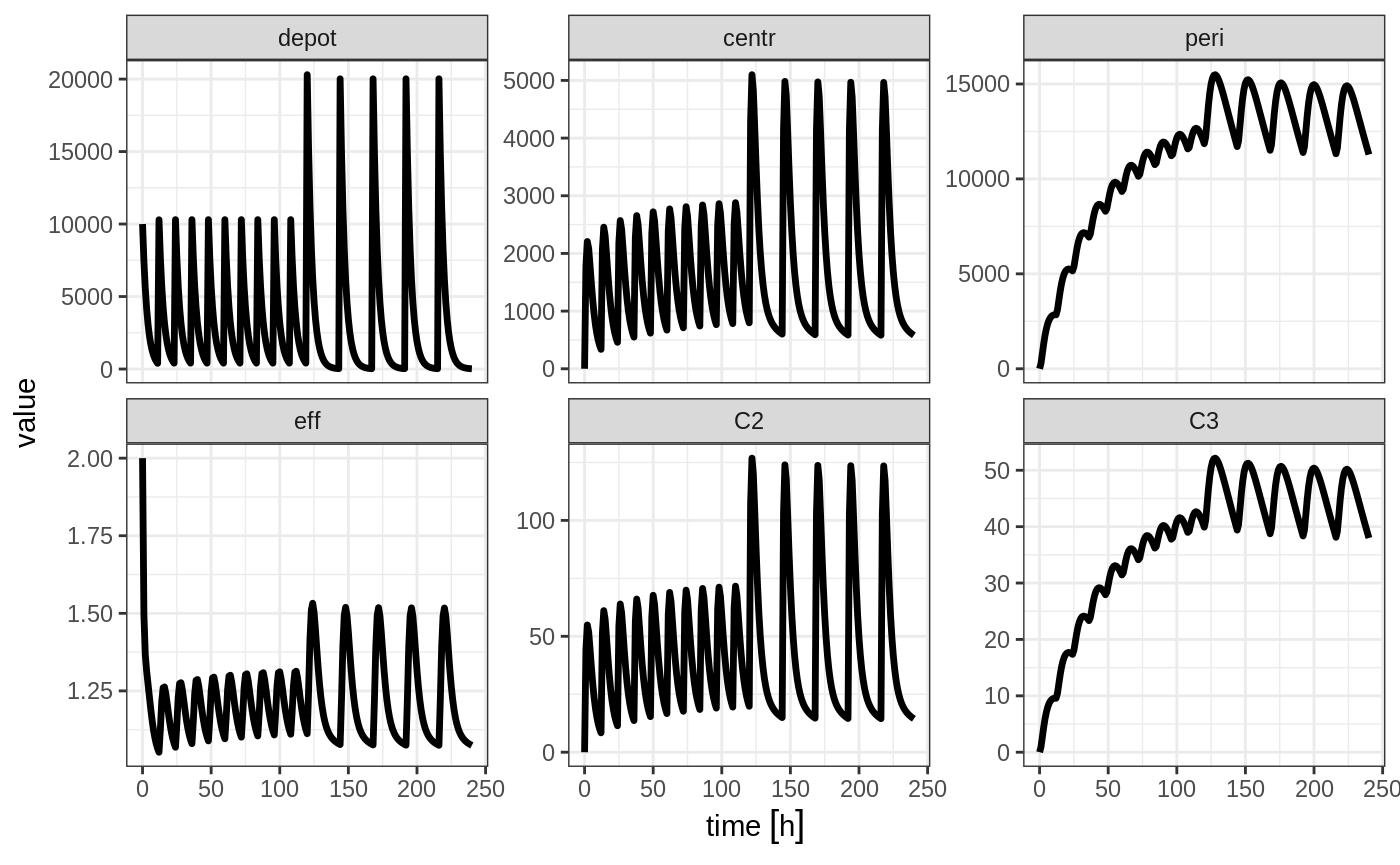
Modifying observation times for RxODE
Notice that the initial effect is now 2.
You can also change the sampling times easily by this method by changing t or time. For example:
x$t <- seq(0,5,length.out=20)
print(x)
#> ___________________________ Solved RxODE object ___________________________
#> -- Parameters ($params): --------------------------------------------------
#>
#>      V2      V3      KA      CL       Q     Kin    Kout    EC50
#>  40.200 297.000   0.294  18.600  10.500   1.000   1.000 200.000
#> -- Initial Conditions ($inits): -------------------------------------------
#> depot centr  peri   eff
#>     0     0     0     2
#> -- First part of data (object): -------------------------------------------
#> # A tibble: 20 x 7
#>        time    C2     C3  depot centr  peri   eff
#>         [h] <dbl>  <dbl>  <dbl> <dbl> <dbl> <dbl>
#> 1 0.0000000   0   0      10000     0    0    2
#> 2 0.2631579  16.8 0.0817  9255.  677.  24.3  1.79
#> 3 0.5263158  29.5 0.299   8566. 1187.  88.7  1.65
#> 4 0.7894737  38.9 0.615   7929. 1562. 183.   1.55
#> 5 1.0526316  45.5 1.00    7338. 1830. 298.   1.49
#> 6 1.3157895  50.1 1.44    6792. 2013. 427.   1.44
#> # ... with 14 more rows
#> ___________________________________________________________________________
plot(x)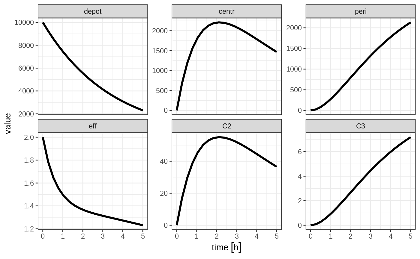
Modifying simulation parameters
You can also access or change parameters by the $ operator. For example, accessing KA can be done by:
x$KA
#> [1] 0.294
And you may change it by assigning it to a new value.
x$KA <- 1;
print(x)
#> ___________________________ Solved RxODE object ___________________________
#> -- Parameters ($params): --------------------------------------------------
#>
#>    V2    V3    KA    CL     Q   Kin  Kout  EC50
#>  40.2 297.0   1.0  18.6  10.5   1.0   1.0 200.0
#> -- Initial Conditions ($inits): -------------------------------------------
#> depot centr  peri   eff
#>     0     0     0     2
#> -- First part of data (object): -------------------------------------------
#> # A tibble: 20 x 7
#>        time    C2    C3  depot centr   peri   eff
#>         [h] <dbl> <dbl>  <dbl> <dbl>  <dbl> <dbl>
#> 1 0.0000000   0   0     10000     0     0    2
#> 2 0.2631579  52.2 0.261  7686. 2098.   77.6  1.82
#> 3 0.5263158  83.3 0.900  5908. 3348.  267.   1.74
#> 4 0.7894737  99.8 1.75   4541. 4010.  519.   1.69
#> 5 1.0526316 106.  2.69   3490. 4273.  800.   1.67
#> 6 1.3157895 106.  3.66   2683. 4272. 1086.   1.64
#> # ... with 14 more rows
#> ___________________________________________________________________________
plot(x)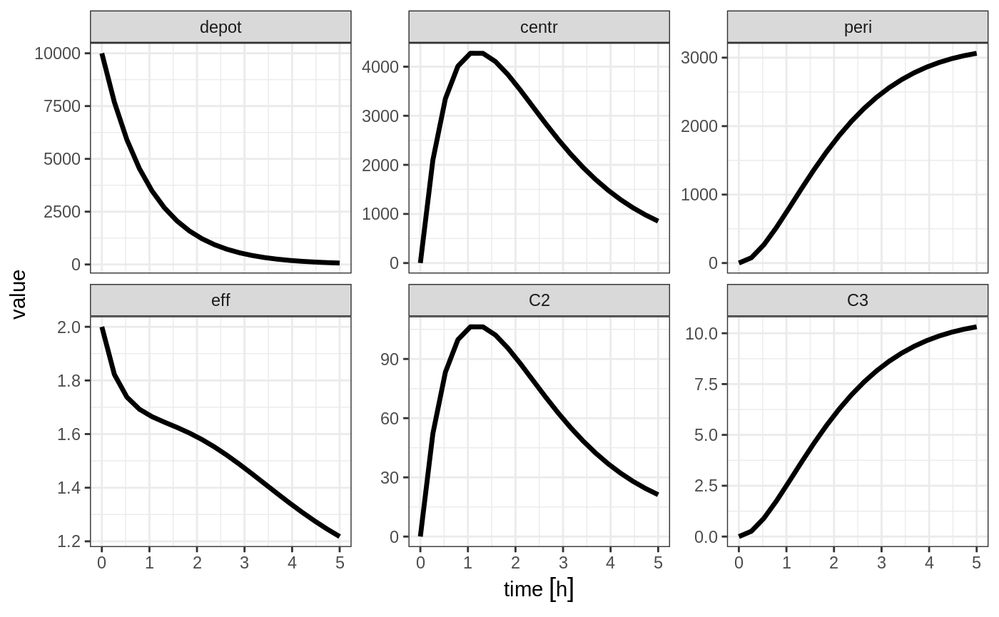
You can access/change all the parameters, initialization(s) or events with the $params, $inits, $events accessor syntax, similar to what is used above.
This syntax makes it easy to update and explore the effect of various parameters on the solved object.