RxODE Covariates

2019-10-16

Covariates are easy to specify in RxODE, you can specify them as a variable. Time-varying covariates, like clock time in a circadian rhythm model, can also be used. Extending the indirect response model already discussed, we have:

library(RxODE)
library(units)

mod3 <- RxODE({
    KA=2.94E-01;
    CL=1.86E+01; 
    V2=4.02E+01; 
    Q=1.05E+01;
    V3=2.97E+02; 
    Kin0=1;
    Kout=1;
    EC50=200;
    ## The linCmt() picks up the variables from above
    C2   = linCmt();
    Tz= 8
    amp=0.1
    eff(0) = 1  ## This specifies that the effect compartment starts at 1.
    ## Kin changes based on time of day (like cortosol)
    Kin =   Kin0 +amp *cos(2*pi*(ctime-Tz)/24)
    d/dt(eff) =  Kin - Kout*(1-C2/(EC50+C2))*eff;
})


ev <- eventTable(amount.units="mg", time.units="hours") %>%
    add.dosing(dose=10000, nbr.doses=1, dosing.to=2) %>%
    add.sampling(seq(0,48,length.out=100));


## Create data frame of  8 am dosing for the first dose
ev$ctime <- (ev$time+set_units(8,hr)) %% 24

Now there is a covariate present, the system can be solved using the cov option

r1 <- solve(mod3, ev, covs_interpolation="linear")
print(r1)
#> ▂▂▂▂▂▂▂▂▂▂▂▂▂▂▂▂▂▂▂▂▂▂▂▂▂▂▂ Solved RxODE object ▂▂▂▂▂▂▂▂▂▂▂▂▂▂▂▂▂▂▂▂▂▂▂▂▂▂▂
#> ── Parameters ($params): ──────────────────────────────────────────────────
#>  
#>         KA         CL         V2          Q         V3       Kin0 
#>   0.294000  18.600000  40.200000  10.500000 297.000000   1.000000 
#>       Kout       EC50         Tz        amp         pi 
#>   1.000000 200.000000   8.000000   0.100000   3.141593 
#> ── Initial Conditions ($inits): ───────────────────────────────────────────
#> eff 
#>   1 
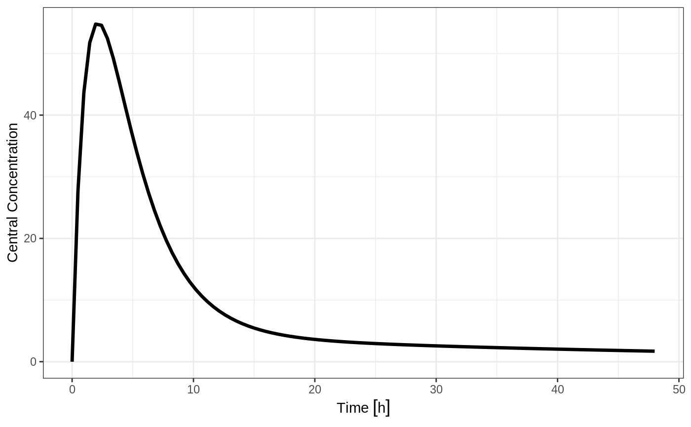
#> ── First part of data (object): ───────────────────────────────────────────
#> # A tibble: 100 x 4
#>        time    C2   Kin   eff
#>         [h] <dbl> <dbl> <dbl>
#> 1 0.0000000   0    1.1   1   
#> 2 0.4848485  27.8  1.10  1.07
#> 3 0.9696970  43.7  1.10  1.15
#> 4 1.4545455  51.8  1.09  1.22
#> 5 1.9393939  54.8  1.09  1.27
#> 6 2.4242424  54.6  1.08  1.30
#> # … with 94 more rows
#> ▂▂▂▂▂▂▂▂▂▂▂▂▂▂▂▂▂▂▂▂▂▂▂▂▂▂▂▂▂▂▂▂▂▂▂▂▂▂▂▂▂▂▂▂▂▂▂▂▂▂▂▂▂▂▂▂▂▂▂▂▂▂▂▂▂▂▂▂▂▂▂▂▂▂▂

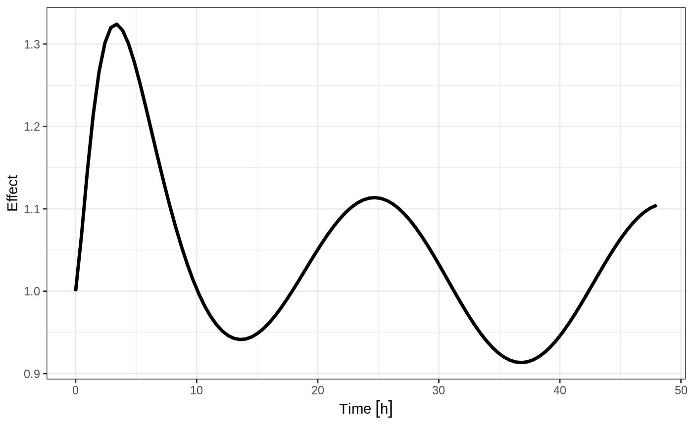
When solving ODE equations, the solver may sample times outside of the data. When this happens, this ODE solver uses linear interpolation between the covariate values. This is the default value. It is equivalent to R’s approxfun with method="linear", which is the default approxfun.

library(ggplot2)
plot(r1,C2) +ylab("Central Concentration") + xlab("Time");

plot(r1,eff) + ylab("Effect") + xlab("Time");

Note that the linear approximation in this case leads to some kinks in the solved system at 24-hours where the covariate has a linear interpolation between near 24 and near 0.

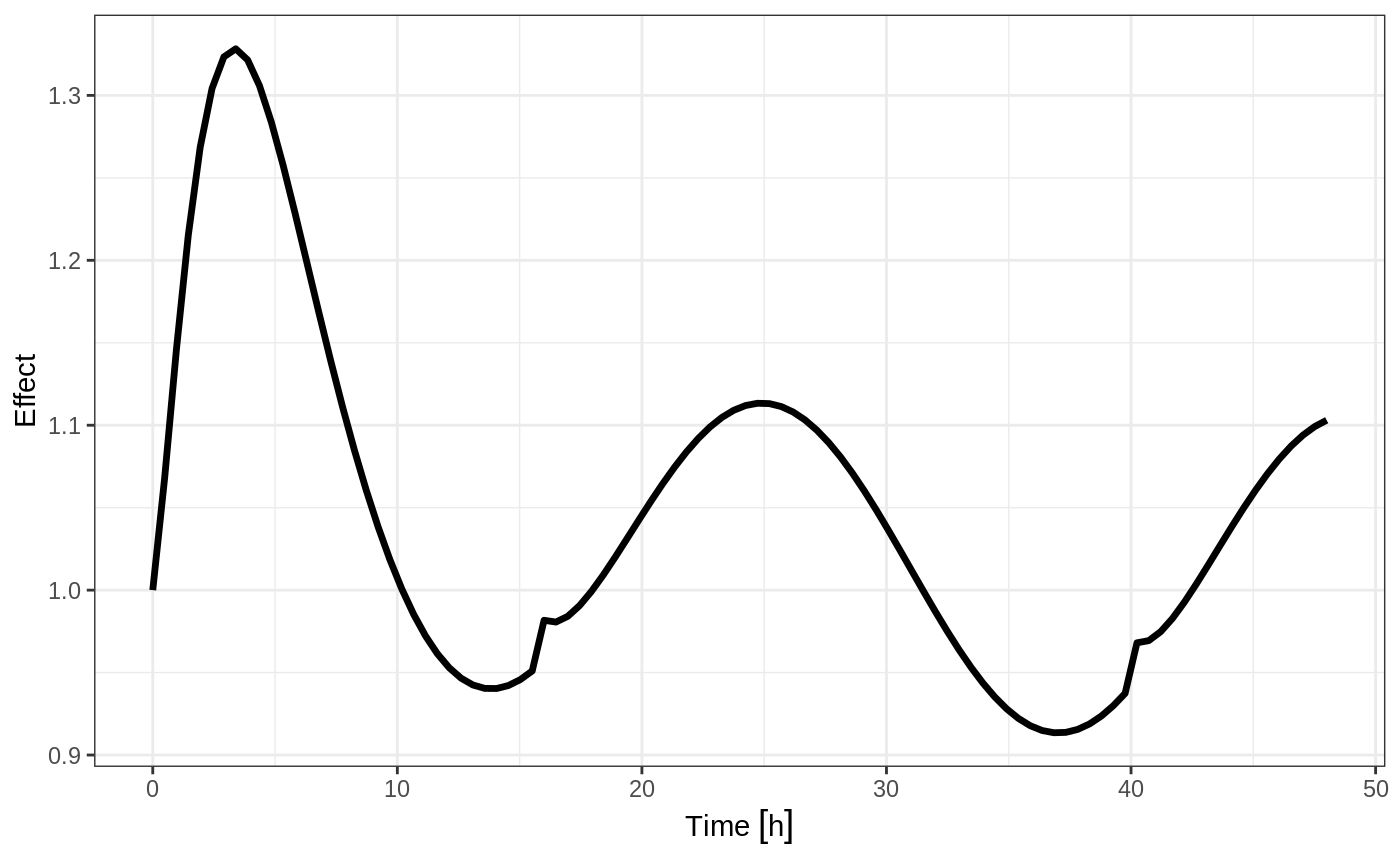
In RxODE, covariate interpolation can also be the last observation carried forward, or constant approximation. This is equivalent to R’s approxfun with method="constant".

r1 <- solve(mod3, ev,covs_interpolation="constant")
print(r1)
#> ▂▂▂▂▂▂▂▂▂▂▂▂▂▂▂▂▂▂▂▂▂▂▂▂▂▂▂ Solved RxODE object ▂▂▂▂▂▂▂▂▂▂▂▂▂▂▂▂▂▂▂▂▂▂▂▂▂▂▂
#> ── Parameters ($params): ──────────────────────────────────────────────────
#>  
#>         KA         CL         V2          Q         V3       Kin0 
#>   0.294000  18.600000  40.200000  10.500000 297.000000   1.000000 
#>       Kout       EC50         Tz        amp         pi 
#>   1.000000 200.000000   8.000000   0.100000   3.141593 
#> ── Initial Conditions ($inits): ───────────────────────────────────────────
#> eff 
#>   1 
#> ── First part of data (object): ───────────────────────────────────────────
#> # A tibble: 100 x 4
#>        time    C2   Kin   eff
#>         [h] <dbl> <dbl> <dbl>
#> 1 0.0000000   0    1.1   1   
#> 2 0.4848485  27.8  1.10  1.07
#> 3 0.9696970  43.7  1.10  1.15
#> 4 1.4545455  51.8  1.09  1.22
#> 5 1.9393939  54.8  1.09  1.27
#> 6 2.4242424  54.6  1.08  1.31
#> # … with 94 more rows
#> ▂▂▂▂▂▂▂▂▂▂▂▂▂▂▂▂▂▂▂▂▂▂▂▂▂▂▂▂▂▂▂▂▂▂▂▂▂▂▂▂▂▂▂▂▂▂▂▂▂▂▂▂▂▂▂▂▂▂▂▂▂▂▂▂▂▂▂▂▂▂▂▂▂▂▂

which gives the following plots:

plot(r1,C2) + ylab("Central Concentration") + xlab("Time");

plot(r1,eff) + ylab("Effect") + xlab("Time");

In this case, the plots seem to be smoother.

You can also use NONMEM’s preferred interpolation style of next observation carried backward (NOCB):

r1 <- solve(mod3, ev,covs_interpolation="nocb")
print(r1)
#> ▂▂▂▂▂▂▂▂▂▂▂▂▂▂▂▂▂▂▂▂▂▂▂▂▂▂▂ Solved RxODE object ▂▂▂▂▂▂▂▂▂▂▂▂▂▂▂▂▂▂▂▂▂▂▂▂▂▂▂
#> ── Parameters ($params): ──────────────────────────────────────────────────
#>  
#>         KA         CL         V2          Q         V3       Kin0 
#>   0.294000  18.600000  40.200000  10.500000 297.000000   1.000000 
#>       Kout       EC50         Tz        amp         pi 
#>   1.000000 200.000000   8.000000   0.100000   3.141593 
#> ── Initial Conditions ($inits): ───────────────────────────────────────────
#> eff 
#>   1 
#> ── First part of data (object): ───────────────────────────────────────────
#> # A tibble: 100 x 4
#>        time    C2   Kin   eff
#>         [h] <dbl> <dbl> <dbl>
#> 1 0.0000000   0    1.1   1   
#> 2 0.4848485  27.8  1.10  1.07
#> 3 0.9696970  43.7  1.10  1.15
#> 4 1.4545455  51.8  1.09  1.21
#> 5 1.9393939  54.8  1.09  1.27
#> 6 2.4242424  54.6  1.08  1.30
#> # … with 94 more rows
#> ▂▂▂▂▂▂▂▂▂▂▂▂▂▂▂▂▂▂▂▂▂▂▂▂▂▂▂▂▂▂▂▂▂▂▂▂▂▂▂▂▂▂▂▂▂▂▂▂▂▂▂▂▂▂▂▂▂▂▂▂▂▂▂▂▂▂▂▂▂▂▂▂▂▂▂

which gives the following plots:

plot(r1,C2) + ylab("Central Concentration") + xlab("Time");

plot(r1,eff) + ylab("Effect") + xlab("Time");