RxODE Events
2019-10-16
RxODE-events.Rmd
RxODE event tables
In general, RxODE event tables follow NONMEM convention with the exceptions:
- The compartment data item (
cmt) can be a string/factor with compartment names - You may turn off a compartment with a negative compartment number or “-cmt” where cmt is the compartment name.
- The compartment data item (
cmt) can still be a number, the number of the compartment is defined by the appearance of the compartment name in the model. This can be tedious to count, so you can specify compartment numbers easier by using thecmt(cmtName)at the beginning of the model. - An additional column,
durcan specify the duration of infusions;- Bioavailability changes will change the rate of infusion since
dur/amtare fixed in the input data. - Similarly, when specifying
rate/amtfor an infusion, the bioavailability will change the infusion duration sincerate/amtare fixed in the input data.
- Bioavailability changes will change the rate of infusion since
- Some infrequent NONMEM columns are not supported:
pcmt,call. - Additional events are supported:
-
evid=5or replace event; This replaces the value of a compartment with the value specified in theamtcolumn. This is equivalent todeSolve=replace. -
evid=6or multiply event; This multiplies the value in the compartment with the value specified by theamtcolumn. This is equivalent todeSolve=multiply.
Here are the legal entries to a data table:
| Data Item | Meaning | Notes |
|---|---|---|
| id | Individual identifier | Must be an integer > 0, sorted |
| time | Individual time | For each ID must be ascending and non-negative |
| amt | dose amount | Positive for doses zero/NA for observations |
| rate | infusion rate | When specified the infusion duration will be dur=amt/rate |
| rate = -1, rate modeled; rate = -2, duration modeled | ||
| dur | infusion duration | When specified the infusion rate will be rate = amt/dur |
| evid | event ID | 0=Observation; 1=Dose; 2=Other; 3=Reset; 4=Reset+Dose; 5=Replace; 6=Multiply |
| cmt | Compartment | Represents compartment #/name for dose/observation |
| ss | Steady State Flag | 0 = non-steady-state; 1=steady state; 2=steady state +prior states |
| ii | Inter-dose Interval | Time between doses. |
| addl | # of additional doses | Number of doses like the current dose. |
Other notes:
- The
evidcan be the classic RxODE (described at the end of this document) or the NONMEM-style evid described above. - NONMEM’s
DVis not required; RxODE is a ODE solving framework. - NONMEM’s
MDVis not required, since it is captured inEVID - Instead of NONMEM-compatible data, it can accept
deSolvecompatible data-frames
When returning the RxODE solved data-set there are a few additional event ids (EVID):
- EVID = -1 is when a modeled rate ends (corresponds to rate = -1)
- EVID = -2 is when a modeled duration ends (corresponds to rate=-2)
- EVID = -10 when a rate specified zero-order infusion ends (corresponds to rate > 0)
- EVID = -20 when a duration specified zero-order infusion ends (corresponds to dur > 0)
- EVID = 101, 102, 103,… These correspond to the 1, 2, 3, … modeled time (mtime).
These can only be accessed when solving with the option combination addDosing=TRUE and subsetNonmem=FALSE. If you want to see the classic EVID equivalents you can use addDosing=NA.
Creating RxODE’s event tables
An event table in RxODE is a specialized data frame that acts as a container for all of RxODE’s events and observation times.
To create an RxODE event table you may use the code eventTable(), et(), or even create your own data frame with the right event information contained in it.
library(RxODE)
(ev <- eventTable());
#> --------------------------- EventTable with 0 records --------------------------
#> 0 dosing records (see x$get.dosing(); add with add.dosing or et)
#> 0 observation times (see x$get.sampling(); add with add.sampling or et)
#> --------------------------------------------------------------------------------or
(ev <- et());#> --------------------------- EventTable with 0 records --------------------------
#> 0 dosing records (see x$get.dosing(); add with add.dosing or et)
#> 0 observation times (see x$get.sampling(); add with add.sampling or et)
#> --------------------------------------------------------------------------------For these models, we can illustrate by using the model shared in the RxODE tutorial:
## Model from RxODE tutorial
m1 <-RxODE({
    KA=2.94E-01;
    CL=1.86E+01;
    V2=4.02E+01;
    Q=1.05E+01;
    V3=2.97E+02;
    Kin=1;
    Kout=1;
    EC50=200;
    ## Added modeled bioavaiblity, duration and rate
    fdepot = 1;
    durDepot = 8;
    rateDepot = 1250;
    C2 = centr/V2;
    C3 = peri/V3;
    d/dt(depot) =-KA*depot;
    f(depot) = fdepot
    dur(depot) = durDepot
    rate(depot) = rateDepot
    d/dt(centr) = KA*depot - CL*C2 - Q*C2 + Q*C3;
    d/dt(peri)  =                    Q*C2 - Q*C3;
    d/dt(eff)  = Kin - Kout*(1-C2/(EC50+C2))*eff;
    eff(0) = 1
});
Adding doses to the event table
Once created you can add dosing to the event table by the add.dosing, and et functions.
Using the add.dosing function you have:
| argument | meaning |
|---|---|
| dose | dose amount |
| nbr.doses | Number of doses; Should be at least 1. |
| dosing.interval | Dosing interval; By default this is 24. |
| dosing.to | Compartment where dose is administered. |
| rate | Infusion rate |
| start.time | The start time of the dose |
ev <- eventTable(amount.units="mg", time.units="hr")

## The methods ar attached to the event table, so you can use them
## directly
ev$add.dosing(dose=10000, nbr.doses = 3)# loading doses
## Starts at time 0; Default dosing interval is 24

## You can also pipe the event tables to these methods.
ev <- ev %>%
    add.dosing(dose=5000, nbr.doses=14, dosing.interval=12)# maintenance

ev
#> --------------------------- EventTable with 2 records --------------------------
#> 2 dosing records (see x$get.dosing(); add with add.dosing or et)
#> 0 observation times (see x$get.sampling(); add with add.sampling or et)
#> multiple doses in `addl` columns, expand with x$expand(); or etExpand(x)
#> -- First part of x: ------------------------------------------------------------
#> # A tibble: 2 x 5
#> time amt ii addl evid
#> [h] [mg] [h] <int> <evid>
#> 1 0 10000 24 2 1:Dose (Add)
#> 2 0 5000 12 13 1:Dose (Add)
#> --------------------------------------------------------------------------------Notice that the units were specified in the table. When specified, the units use the units package to keep track of the units and convert them if needed. Additionally, ggforce uses them to label the ggplot axes. The set_units and drop_units are useful to set and drop the RxODE event table units.
In this example, you can see the time axes is labeled:
If you are more familiar with the NONMEM/RxODE event records, you can also specify dosing using et with the dose elements directly:
#> --------------------------- EventTable with 1 records --------------------------
#>    1 dosing records (see x$get.dosing(); add with add.dosing or et)
#>    0 observation times (see x$get.sampling(); add with add.sampling or et)
#>    multiple doses in `addl` columns, expand with x$expand(); or etExpand(x)
#> -- First part of x: ------------------------------------------------------------
#> # A tibble: 1 x 5
#>    time   amt    ii  addl evid
#>     [h] <dbl>   [h] <int> <evid>
#> 1     0 10000    12     6 1:Dose (Add)
#> --------------------------------------------------------------------------------
Which gives:
This shows how easy creating event tables can be.
Adding sampling to an event table
If you notice in the above examples, RxODE generated some default sampling times since there was not any sampling times. If you wish more control over the sampling time, you should add the samples to the RxODE event table by add.sampling or et
ev <- eventTable(amount.units="mg", time.units="hr")

## The methods ar attached to the event table, so you can use them
## directly
ev$add.dosing(dose=10000, nbr.doses = 3)# loading doses

ev$add.sampling(seq(0,24,by=4))

ev
#> --------------------------- EventTable with 8 records --------------------------
#> 1 dosing records (see x$get.dosing(); add with add.dosing or et)
#> 7 observation times (see x$get.sampling(); add with add.sampling or et)
#> multiple doses in `addl` columns, expand with x$expand(); or etExpand(x)
#> -- First part of x: ------------------------------------------------------------
#> # A tibble: 8 x 5
#> time amt ii addl evid
#> [h] [mg] [h] <int> <evid>
#> 1 0 NA NA NA 0:Observation
#> 2 0 10000 24 2 1:Dose (Add)
#> 3 4 NA NA NA 0:Observation
#> 4 8 NA NA NA 0:Observation
#> 5 12 NA NA NA 0:Observation
#> 6 16 NA NA NA 0:Observation
#> 7 20 NA NA NA 0:Observation
#> 8 24 NA NA NA 0:Observation
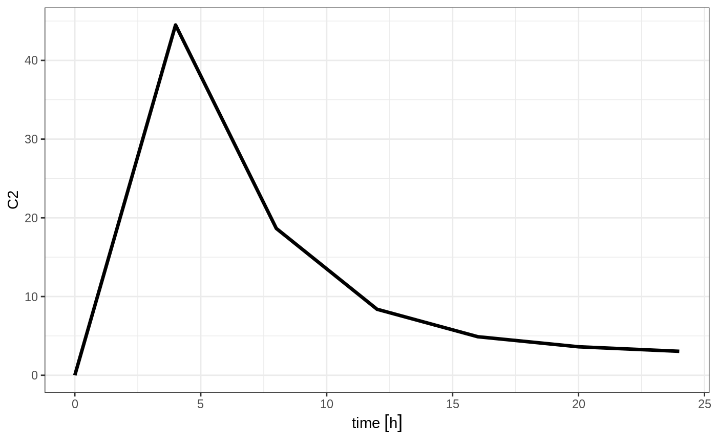
#> --------------------------------------------------------------------------------Which gives:
Or if you use et you can simply add them in a similar way to add.sampling:
ev <- et(timeUnits="hr") %>%
    et(amt=10000, until = set_units(3, days), ii=12) %>% # loading doses
    et(seq(0,24,by=4))

ev
#> --------------------------- EventTable with 8 records --------------------------
#> 1 dosing records (see x$get.dosing(); add with add.dosing or et)
#> 7 observation times (see x$get.sampling(); add with add.sampling or et)
#> multiple doses in `addl` columns, expand with x$expand(); or etExpand(x)
#> -- First part of x: ------------------------------------------------------------
#> # A tibble: 8 x 5
#> time amt ii addl evid
#> [h] <dbl> [h] <int> <evid>
#> 1 0 NA NA NA 0:Observation
#> 2 0 10000 12 6 1:Dose (Add)
#> 3 4 NA NA NA 0:Observation
#> 4 8 NA NA NA 0:Observation
#> 5 12 NA NA NA 0:Observation
#> 6 16 NA NA NA 0:Observation
#> 7 20 NA NA NA 0:Observation
#> 8 24 NA NA NA 0:Observation
#> --------------------------------------------------------------------------------which gives the following RxODE solve:
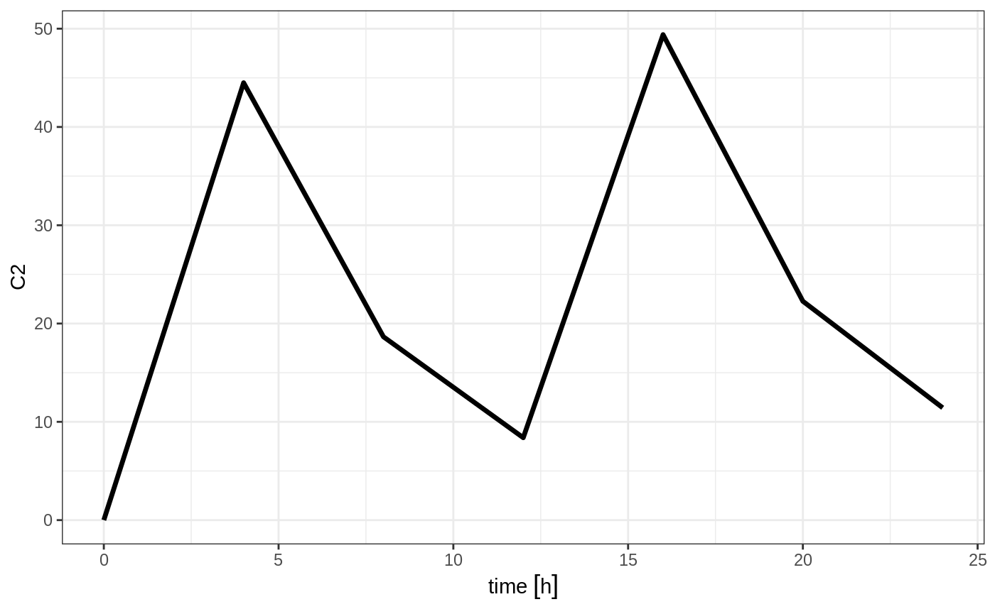
Note the jagged nature of these plots since there was only a few sample times.
Expand the event table to a multi-subject event table.
The only thing that is needed to expand an event table is a list of IDs that you want to expand;
ev <- et(timeUnits="hr") %>%
    et(amt=10000, until = set_units(3, days), ii=12) %>% # loading doses
    et(seq(0,48,length.out=200)) %>%
    et(id=1:4)

ev
#> -------------------------- EventTable with 804 records -------------------------
#> 4 individuals
#> 4 dosing records (see x$get.dosing(); add with add.dosing or et)
#> 800 observation times (see x$get.sampling(); add with add.sampling or et)
#> multiple doses in `addl` columns, expand with x$expand(); or etExpand(x)
#> -- First part of x: ------------------------------------------------------------
#> # A tibble: 804 x 6
#> id time amt ii addl evid
#> <int> [h] <dbl> [h] <int> <evid>
#> 1 1 0.0000000 NA NA NA 0:Observation
#> 2 1 0.0000000 10000 12 6 1:Dose (Add)
#> 3 1 0.2412060 NA NA NA 0:Observation
#> 4 1 0.4824121 NA NA NA 0:Observation
#> 5 1 0.7236181 NA NA NA 0:Observation
#> 6 1 0.9648241 NA NA NA 0:Observation
#> 7 1 1.2060302 NA NA NA 0:Observation
#> 8 1 1.4472362 NA NA NA 0:Observation
#> 9 1 1.6884422 NA NA NA 0:Observation
#> 10 1 1.9296482 NA NA NA 0:Observation
#> # ... with 794 more rows
#> --------------------------------------------------------------------------------You can see in the following simulation there are 4 individuals that are solved for:
set.seed(42)
solve(m1, ev,
      params=data.frame(KA=0.294*exp(rnorm(4)), 18.6*exp(rnorm(4)))) %>%
    plot(C2)
#> Warning in (function (idData, goodLvl, type = "parameter", warnIdSort) : ID missing in parameters dataset;
#> Parameters are assumed to have the same order as the IDs in the event dataset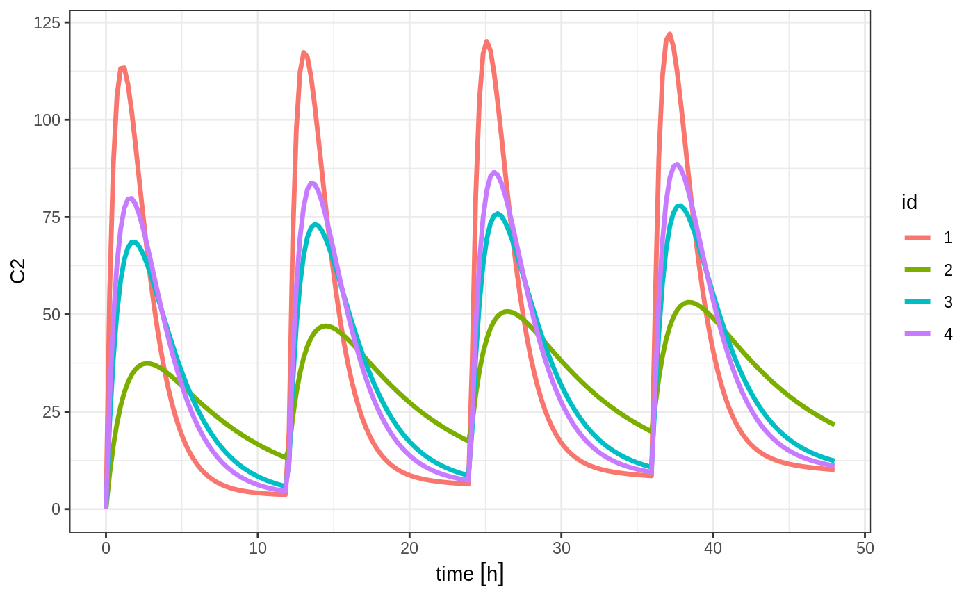
Add doses and samples within a sampling window
In addition to adding fixed doses and fixed sampling times, you can have windows where you sample and draw doses from. For dosing windows you specify the time as an ordered numerical vector with the lowest dosing time and the highest dosing time inside a list.
In this example, you start with a dosing time with a 6 hour dosing window:
set.seed(42)
ev <- et(timeUnits="hr") %>%
    et(time=list(c(0,6)), amt=10000, until = set_units(2, days), ii=12) %>% # loading doses
    et(id=1:4)

ev
#> -------------------------- EventTable with 16 records --------------------------
#> 4 individuals
#> 16 dosing records (see x$get.dosing(); add with add.dosing or et)
#> 0 observation times (see x$get.sampling(); add with add.sampling or et)
#> -- First part of x: ------------------------------------------------------------
#> # A tibble: 16 x 6
#> id low time high amt evid
#> <int> [h] [h] [h] <dbl> <evid>
#> 1 1 0 5.4888363 6 10000 1:Dose (Add)
#> 2 1 12 16.9826858 18 10000 1:Dose (Add)
#> 3 1 24 25.7168372 30 10000 1:Dose (Add)
#> 4 1 36 41.6224525 42 10000 1:Dose (Add)
#> 5 2 0 4.3146735 6 10000 1:Dose (Add)
#> 6 2 12 14.7464507 18 10000 1:Dose (Add)
#> 7 2 24 28.2303887 30 10000 1:Dose (Add)
#> 8 2 36 39.9419537 42 10000 1:Dose (Add)
#> 9 3 0 0.8079996 6 10000 1:Dose (Add)
#> 10 3 12 16.4195299 18 10000 1:Dose (Add)
#> 11 3 24 27.1145757 30 10000 1:Dose (Add)
#> 12 3 36 39.8504731 42 10000 1:Dose (Add)
#> 13 4 0 4.9826858 6 10000 1:Dose (Add)
#> 14 4 12 13.7168372 18 10000 1:Dose (Add)
#> 15 4 24 29.6224525 30 10000 1:Dose (Add)
#> 16 4 36 41.4888363 42 10000 1:Dose (Add)
#> --------------------------------------------------------------------------------You can clearly see different dosing times in the following simulation:
ev <- ev %>% et(seq(0,48,length.out=200))

solve(m1, ev, params=data.frame(KA=0.294*exp(rnorm(4)), 18.6*exp(rnorm(4)))) %>% plot(C2)
#> Warning in (function (idData, goodLvl, type = "parameter", warnIdSort) : ID missing in parameters dataset;
#> Parameters are assumed to have the same order as the IDs in the event dataset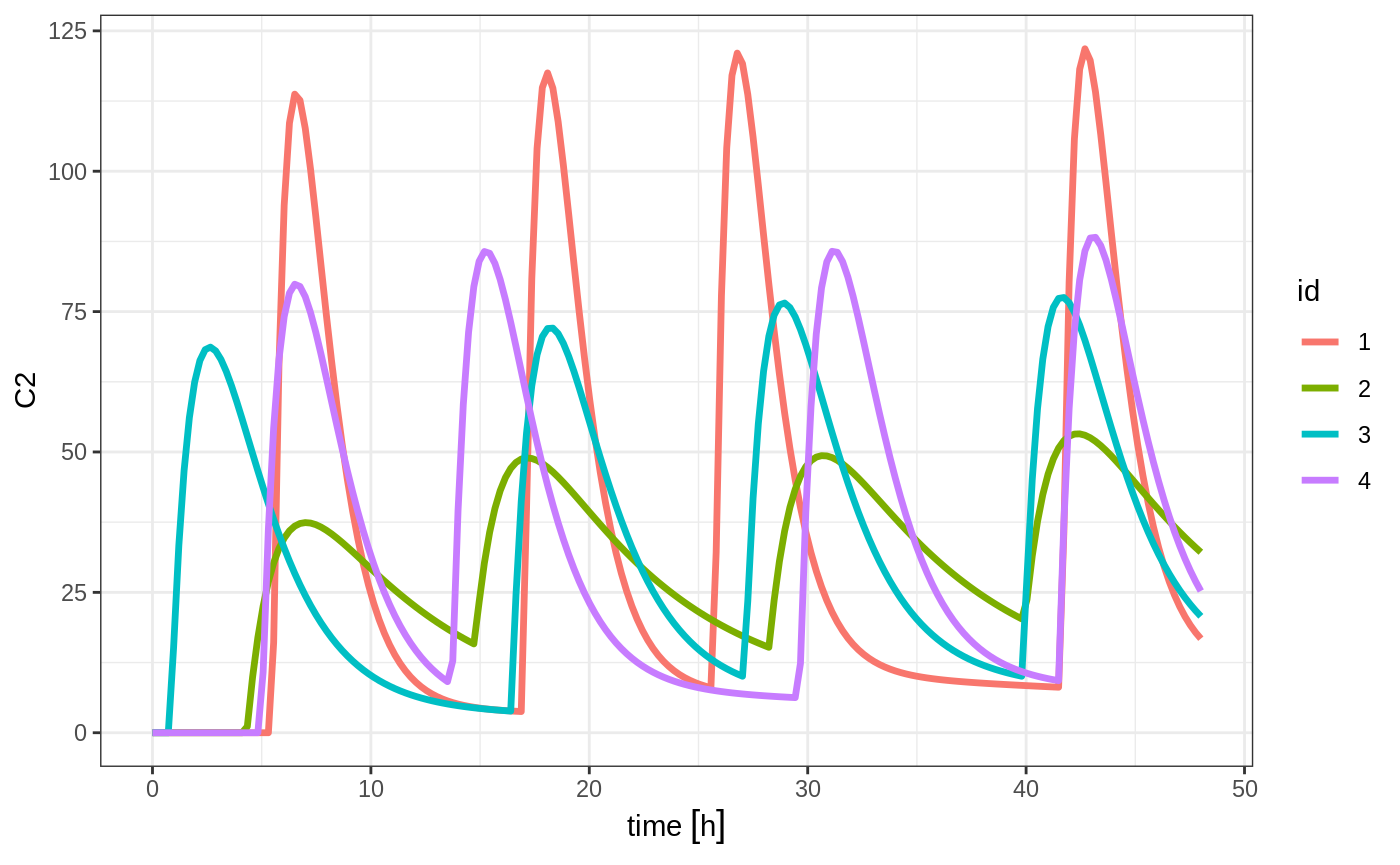
Of course in reality the dosing interval may only be 2 hours:
set.seed(42)
ev <- et(timeUnits="hr") %>%
    et(time=list(c(0,2)), amt=10000, until = set_units(2, days), ii=12) %>% # loading doses
    et(id=1:4) %>%
    et(seq(0,48,length.out=200))

solve(m1, ev, params=data.frame(KA=0.294*exp(rnorm(4)), 18.6*exp(rnorm(4)))) %>% plot(C2)
#> Warning in (function (idData, goodLvl, type = "parameter", warnIdSort) : ID missing in parameters dataset;
#> Parameters are assumed to have the same order as the IDs in the event dataset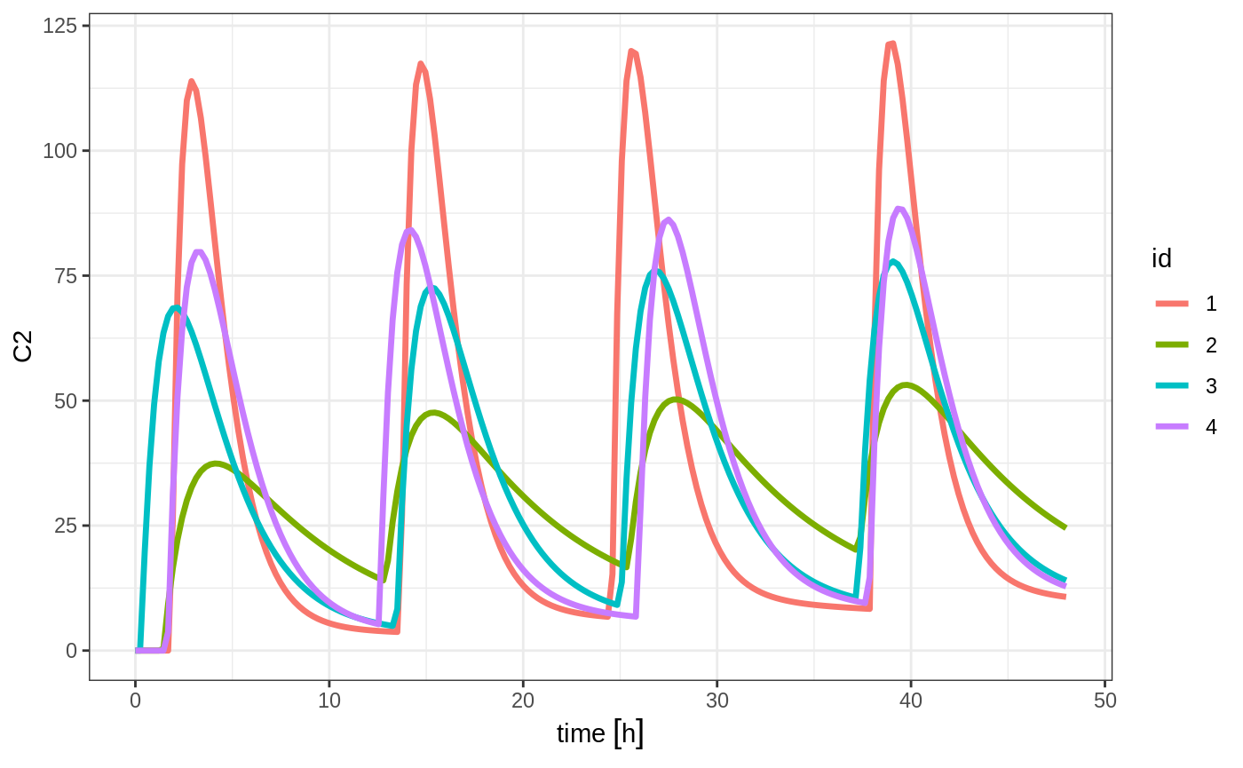
The same sort of thing can be specified with sampling times. To specify the sampling times in terms of a sampling window, you can create a list of the sampling times. Each sampling time will be a two element ordered numeric vector.
set.seed(42)
ev <- et(timeUnits="hr") %>%
    et(time=list(c(0,2)), amt=10000, until = set_units(2, days), ii=12) %>% # loading doses
    et(id=1:4)

## Create 20 samples in the first 24 hours and 20 samples in the second 24 hours
samples <- c(lapply(1:20, function(...){c(0,24)}),
             lapply(1:20, function(...){c(20,48)}))

## Add the random collection to the event table
ev <- ev %>% et(samples)

library(ggplot2)
solve(m1, ev, params=data.frame(KA=0.294*exp(rnorm(4)), 18.6*exp(rnorm(4)))) %>% plot(C2) + geom_point()
#> Warning in (function (idData, goodLvl, type = "parameter", warnIdSort) : ID missing in parameters dataset;
#> Parameters are assumed to have the same order as the IDs in the event dataset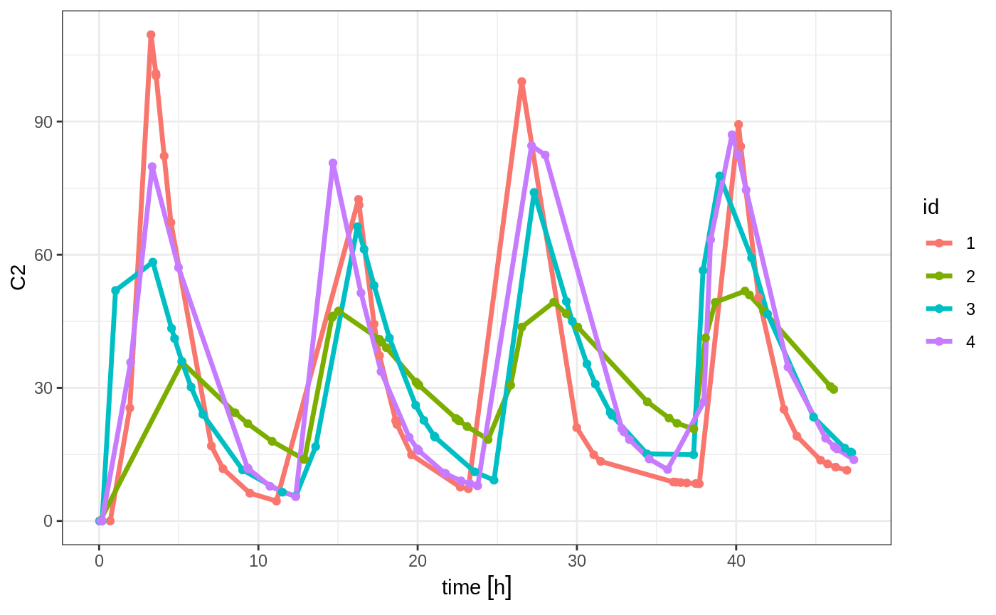
This shows the flexibility in dosing and sampling that the RxODE event tables allow.
Combining event tables
Since you can create dosing records and sampling records, you can create any complex dosing regimen you wish. In addition, RxODE allows you to combine event tables by c, seq, rep, and rbind.
Sequencing event tables
One way to combine event table is to sequence them by c, seq or etSeq. This takes the two dosing groups and adds at least one inter-dose interval between them:
## bid for 5 days
bid <- et(timeUnits="hr") %>%
et(amt=10000,ii=12,until=set_units(5, "days"))
## qd for 5 days
qd <- et(timeUnits="hr") %>%
et(amt=20000,ii=24,until=set_units(5, "days"))
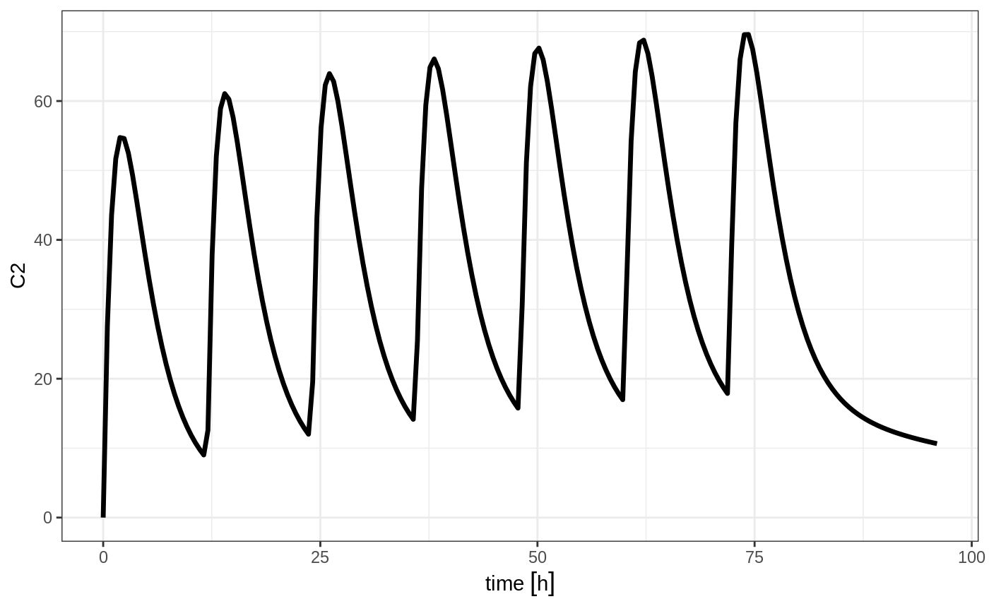
## bid for 5 days followed by qd for 5 days
et <- seq(bid,qd) %>% et(seq(0,11*24,length.out=100));
rxSolve(m1, et) %>% plot(C2)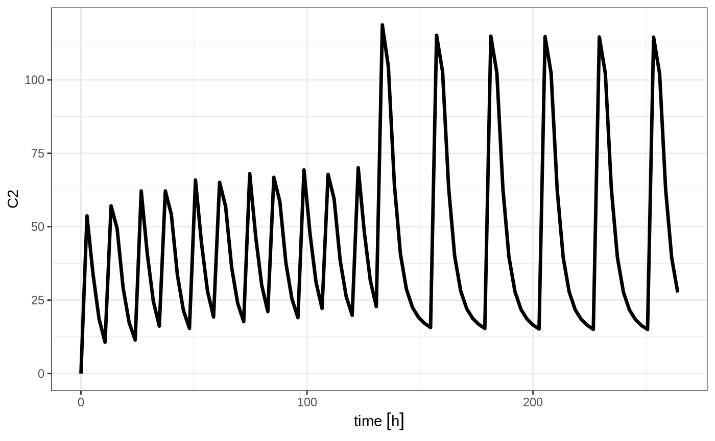
When sequencing events, you can also separate this sequence by a period of time; For example if you wanted to separate this by a week, you could easily do that with the following sequence of event tables:
## bid for 5 days followed by qd for 5 days
et <- seq(bid,set_units(1, "week"), qd) %>%
    et(seq(0,18*24,length.out=100));

rxSolve(m1, et) %>% plot(C2)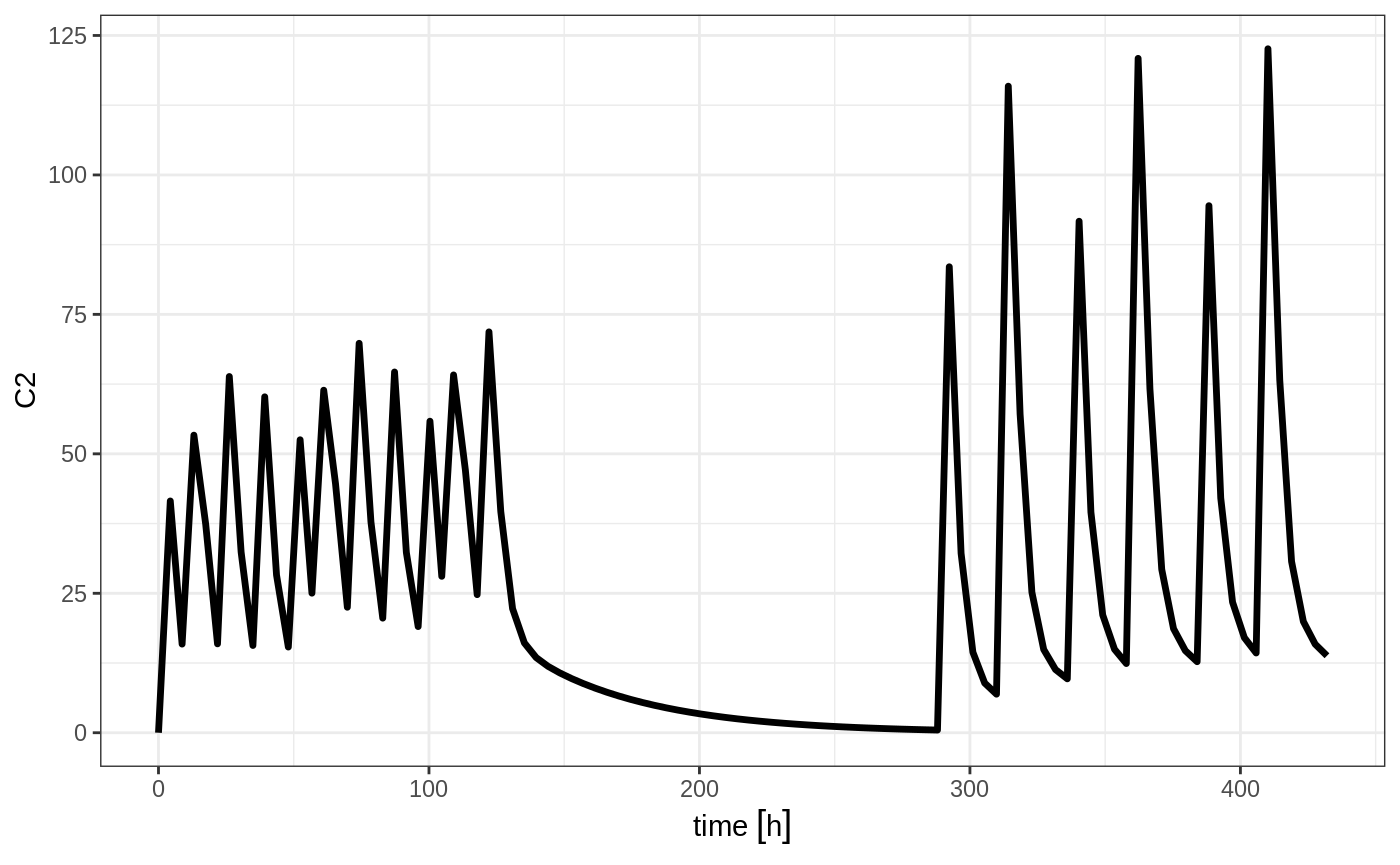
Note that in this example the time between the bid and the qd event tables is exactly one week, not 1 week plus 24 hours because of the inter-dose interval. If you want that behavior, you can sequence it using the wait="+ii".
## bid for 5 days followed by qd for 5 days
et <- seq(bid,set_units(1, "week"), qd,wait="+ii") %>%
    et(seq(0,18*24,length.out=100));

rxSolve(m1, et) %>% plot(C2)
Also note, that RxODE assumes that the dosing is what you want to space the event tables by, and clears out any sampling records when you combine the event tables. If that is not true, you can also use the option samples="use"
Repeating event tables
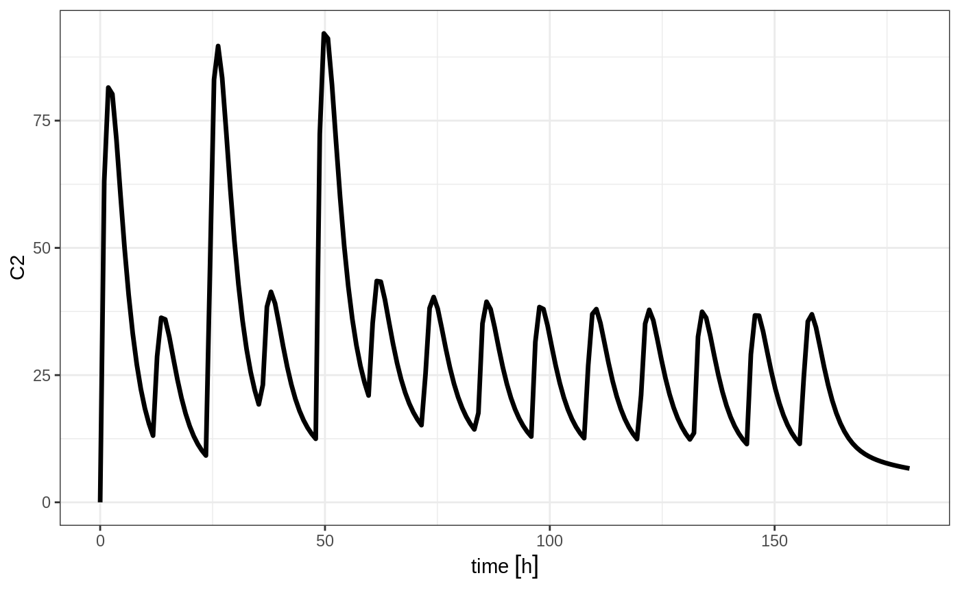
You can have an event table that you can repeat with etRep or rep. For example 4 rounds of 2 weeks on QD therapy and 1 week off of therapy can be simply specified:
qd <-et(timeUnits = "hr") %>% et(amt=10000, ii=24, until=set_units(2, "weeks"), cmt="depot")

et <- rep(qd, times=4, wait=set_units(1,"weeks")) %>%
      add.sampling(set_units(seq(0, 12.5,by=0.005),weeks))

rxSolve(m1, et)  %>% plot(C2)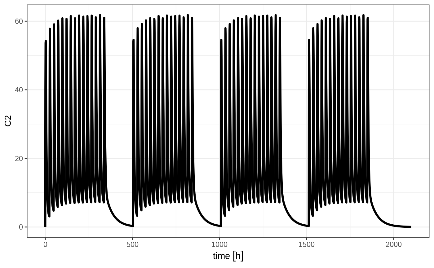
This is a simplified way to use a sequence of event tables. Therefore, many of the same options still apply; That is samples are cleared unless you use samples="use", and the time between event tables is at least the inter-dose interval. You can adjust the timing by the wait option.
Combining event tables with rbind
You may combine event tables with rbind. This does not consider the event times when combining the event tables, but keeps them the same times. If you space the event tables by a waiting period, it also does not consider the inter-dose interval.
Using the previous seq you can clearly see the difference. Here was the sequence:
## bid for 5 days
bid <- et(timeUnits="hr") %>%
       et(amt=10000,ii=12,until=set_units(5, "days"))

## qd for 5 days
qd <- et(timeUnits="hr") %>%
      et(amt=20000,ii=24,until=set_units(5, "days"))

et <- seq(bid,qd) %>%
    et(seq(0,18*24,length.out=500));

rxSolve(m1, et) %>% plot(C2)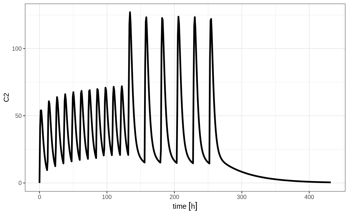
But if you bind them together with rbind
## bid for 5 days
et <- rbind(bid,qd) %>%
    et(seq(0,18*24,length.out=500));

rxSolve(m1, et) %>% plot(C2)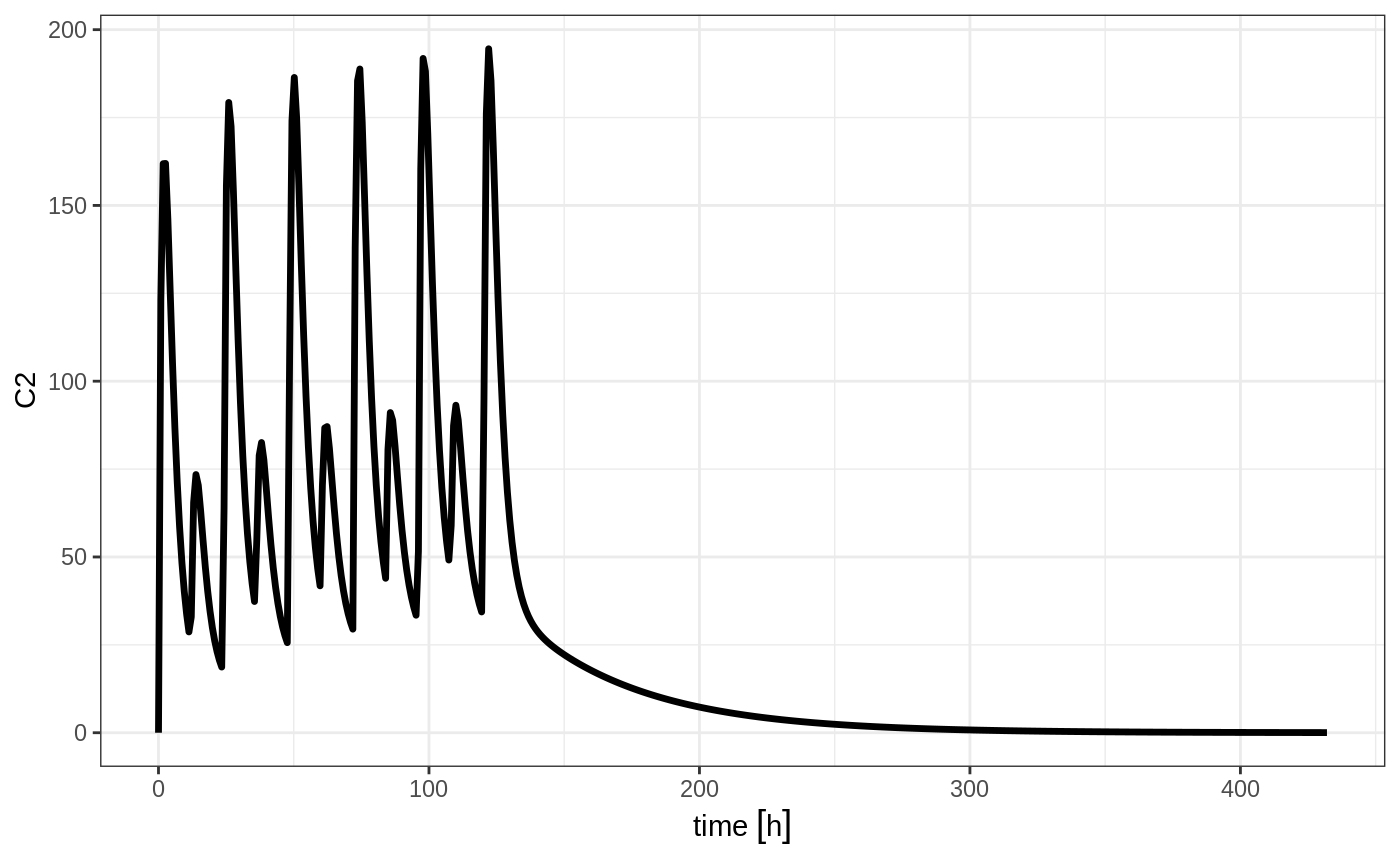
Still the waiting period applies (but does not consider the inter-dose interval)
et <- rbind(bid,wait=set_units(10,days),qd) %>%
    et(seq(0,18*24,length.out=500));

rxSolve(m1, et) %>% plot(C2)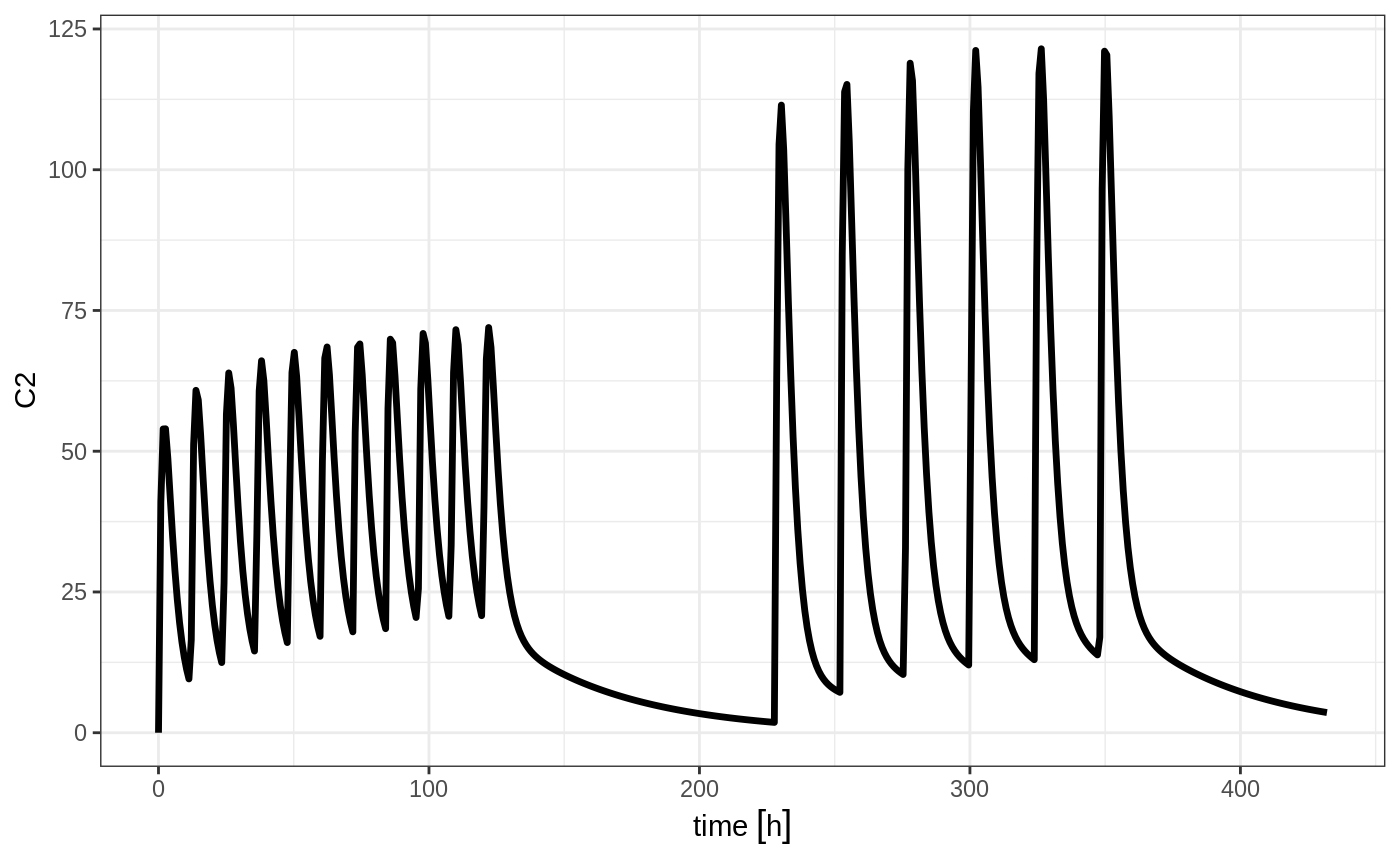
You can also bind the tables together and make each ID in the event table unique; This can be good to combine cohorts with different expected dosing and sampling times. This requires the id="unique" option; Using the first example shows how this is different in this case:
## bid for 5 days
et <- etRbind(bid,qd, id="unique") %>%
    et(seq(0,150,length.out=500));

library(ggplot2)
rxSolve(m1, et) %>% plot(C2) + facet_wrap( ~ id)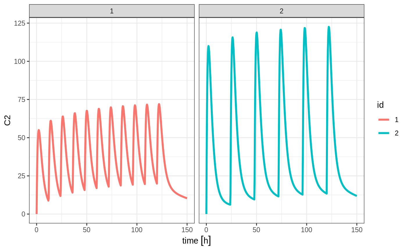
Bolus Doses
A bolus dose is the default type of dose in RxODE and only requires the amt/dose
#> -------------------------- EventTable with 101 records -------------------------
#>    1 dosing records (see x$get.dosing(); add with add.dosing or et)
#>    100 observation times (see x$get.sampling(); add with add.sampling or et)
#>    multiple doses in `addl` columns, expand with x$expand(); or etExpand(x)
#> -- First part of x: ------------------------------------------------------------
#> # A tibble: 101 x 5
#>         time   amt    ii  addl evid
#>          [h] <dbl>   [h] <int> <evid>
#>  1 0.0000000    NA    NA    NA 0:Observation
#>  2 0.0000000 10000    12     2 1:Dose (Add)
#>  3 0.2424242    NA    NA    NA 0:Observation
#>  4 0.4848485    NA    NA    NA 0:Observation
#>  5 0.7272727    NA    NA    NA 0:Observation
#>  6 0.9696970    NA    NA    NA 0:Observation
#>  7 1.2121212    NA    NA    NA 0:Observation
#>  8 1.4545455    NA    NA    NA 0:Observation
#>  9 1.6969697    NA    NA    NA 0:Observation
#> 10 1.9393939    NA    NA    NA 0:Observation
#> # ... with 91 more rows
#> --------------------------------------------------------------------------------
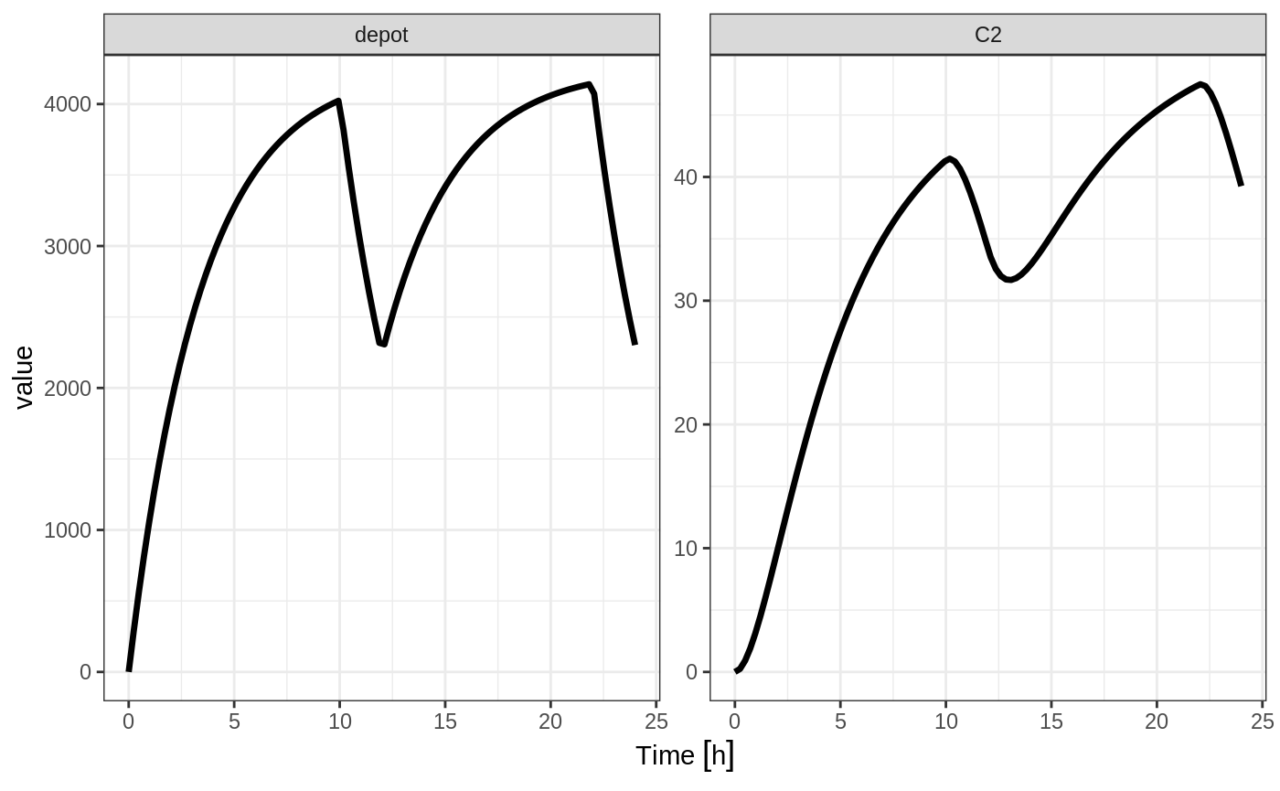
Constant Infusion (in terms of duration and rate)
The next type of event is an infusion; There are two ways to specify an infusion; The first is the dur keyword.
An example of this is:
ev <- et(timeUnits="hr") %>%
    et(amt=10000, ii=12,until=24, dur=8) %>%
    et(seq(0, 24, length.out=100))

ev
#> -------------------------- EventTable with 101 records -------------------------
#> 1 dosing records (see x$get.dosing(); add with add.dosing or et)
#> 100 observation times (see x$get.sampling(); add with add.sampling or et)
#> multiple doses in `addl` columns, expand with x$expand(); or etExpand(x)
#> -- First part of x: ------------------------------------------------------------
#> # A tibble: 101 x 6
#> time amt ii addl evid dur
#> [h] <dbl> [h] <int> <evid> [h]
#> 1 0.0000000 NA NA NA 0:Observation NA
#> 2 0.0000000 10000 12 2 1:Dose (Add) 8
#> 3 0.2424242 NA NA NA 0:Observation NA
#> 4 0.4848485 NA NA NA 0:Observation NA
#> 5 0.7272727 NA NA NA 0:Observation NA
#> 6 0.9696970 NA NA NA 0:Observation NA
#> 7 1.2121212 NA NA NA 0:Observation NA
#> 8 1.4545455 NA NA NA 0:Observation NA
#> 9 1.6969697 NA NA NA 0:Observation NA
#> 10 1.9393939 NA NA NA 0:Observation NA
#> # ... with 91 more rows
#> --------------------------------------------------------------------------------
It can be also specified by the rate component:
ev <- et(timeUnits="hr") %>%
    et(amt=10000, ii=12,until=24, rate=10000/8) %>%
    et(seq(0, 24, length.out=100))

ev
#> -------------------------- EventTable with 101 records -------------------------
#> 1 dosing records (see x$get.dosing(); add with add.dosing or et)
#> 100 observation times (see x$get.sampling(); add with add.sampling or et)
#> multiple doses in `addl` columns, expand with x$expand(); or etExpand(x)
#> -- First part of x: ------------------------------------------------------------
#> # A tibble: 101 x 6
#> time amt rate ii addl evid
#> [h] <dbl> <rate/dur> [h] <int> <evid>
#> 1 0.0000000 NA NA NA NA 0:Observation
#> 2 0.0000000 10000 1250 12 2 1:Dose (Add)
#> 3 0.2424242 NA NA NA NA 0:Observation
#> 4 0.4848485 NA NA NA NA 0:Observation
#> 5 0.7272727 NA NA NA NA 0:Observation
#> 6 0.9696970 NA NA NA NA 0:Observation
#> 7 1.2121212 NA NA NA NA 0:Observation
#> 8 1.4545455 NA NA NA NA 0:Observation
#> 9 1.6969697 NA NA NA NA 0:Observation
#> 10 1.9393939 NA NA NA NA 0:Observation
#> # ... with 91 more rows
#> --------------------------------------------------------------------------------
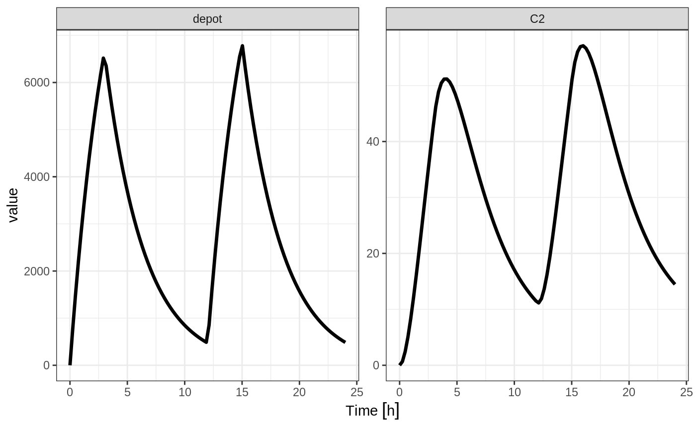
These are the same with the exception of how bioavailability changes the infusion.
In the case of modeling rate, a bioavailability decrease, decreases the infusion duration, as in NONMEM. For example:
Similarly increasing the bioavailability increases the infusion duration.
The rationale for this behavior is that the rate and amt are specified by the event table, so the only thing that can change with a bioavailability increase is the duration of the infusion.
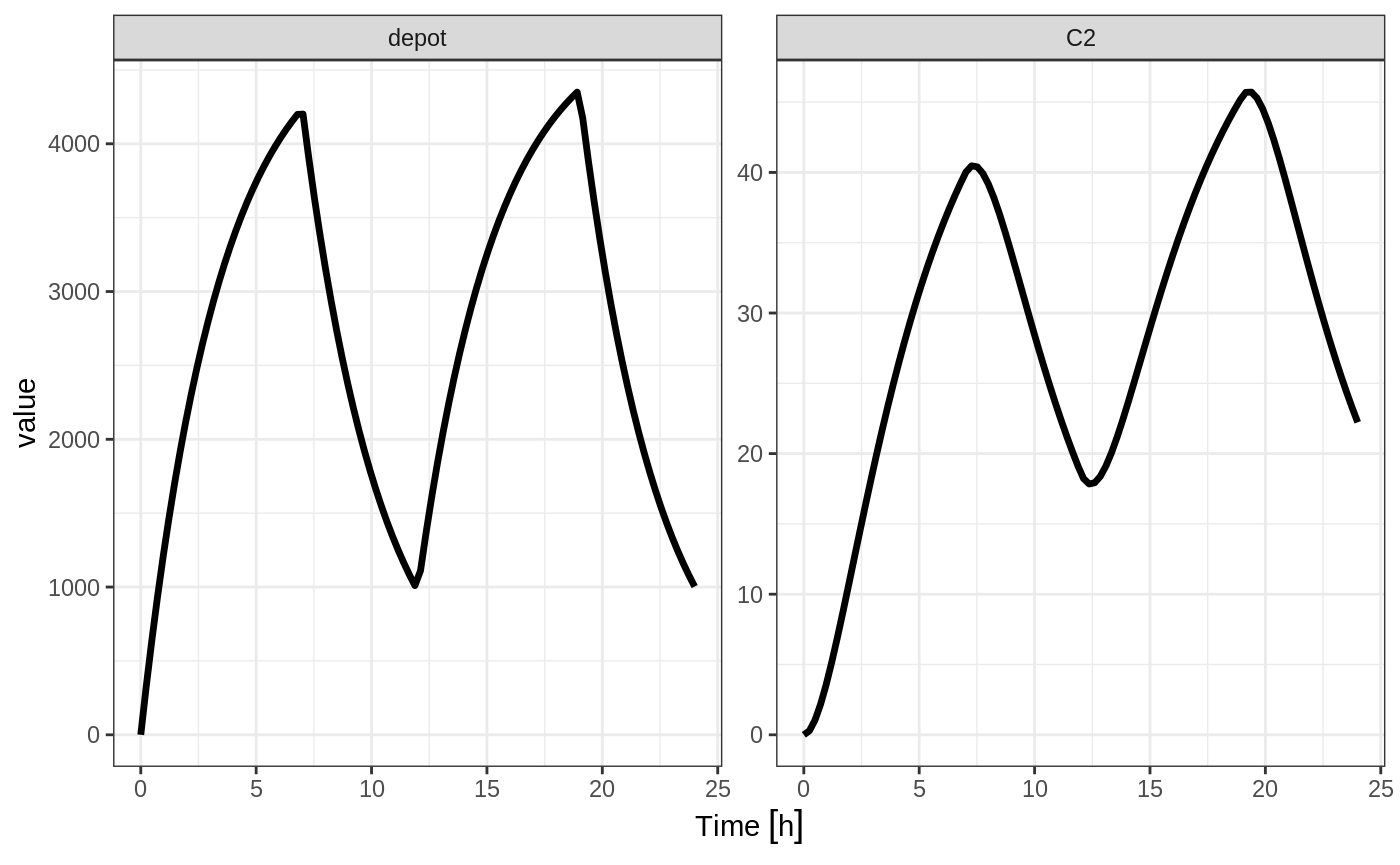
If you specify the amt and dur components in the event table, bioavailability changes affect the rate of infusion.
ev <- et(timeUnits="hr") %>%
    et(amt=10000, ii=12,until=24, dur=8) %>%
    et(seq(0, 24, length.out=100))
You can see the side-by-side comparison of bioavailability changes affecting rate instead of duration with these records in the following plots:
library(ggplot2)
library(gridExtra)

p1 <- rxSolve(m1, ev, c(fdepot=1.25)) %>% plot(depot) +
    xlab("Time") + ylim(0,5000)

p2 <- rxSolve(m1, ev, c(fdepot=0.25)) %>% plot(depot) +
    xlab("Time")+ ylim(0,5000)

grid.arrange(p1,p2, nrow=1)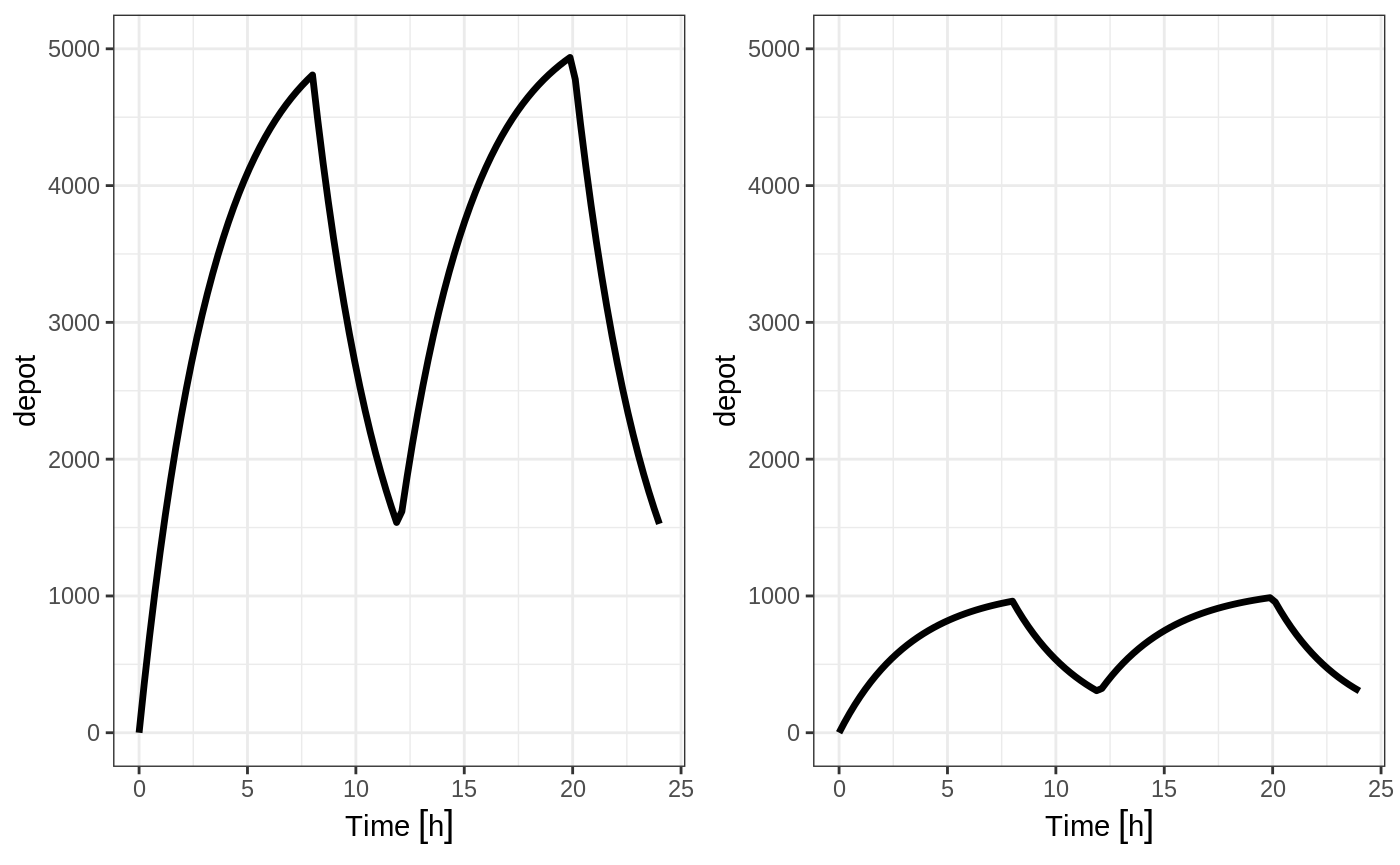
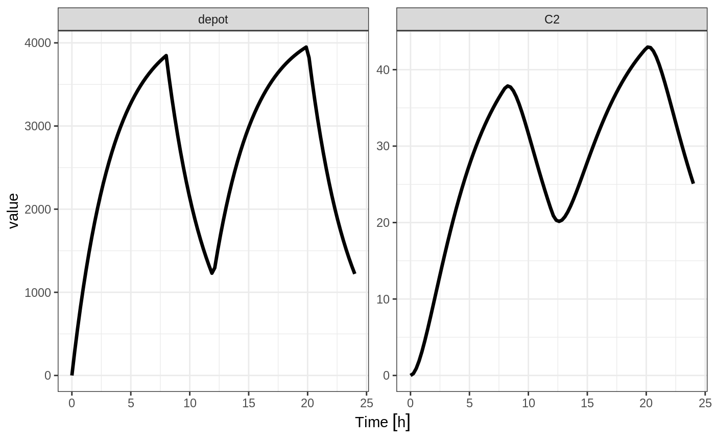
Modeled Rate and Duration of Infusion
You can model the duration, which is equivalent to NONMEM’s rate=-2. As a mnemonic you can use the dur=model instead of rate=-2
ev <- et(timeUnits="hr") %>%
    et(amt=10000, ii=12,until=24, dur=model) %>%
    et(seq(0, 24, length.out=100))

ev
#> -------------------------- EventTable with 101 records -------------------------
#> 1 dosing records (see x$get.dosing(); add with add.dosing or et)
#> 100 observation times (see x$get.sampling(); add with add.sampling or et)
#> multiple doses in `addl` columns, expand with x$expand(); or etExpand(x)
#> -- First part of x: ------------------------------------------------------------
#> # A tibble: 101 x 6
#> time amt rate ii addl evid
#> [h] <dbl> <rate/dur> [h] <int> <evid>
#> 1 0.0000000 NA NA NA NA 0:Observation
#> 2 0.0000000 10000 -2:dur 12 2 1:Dose (Add)
#> 3 0.2424242 NA NA NA NA 0:Observation
#> 4 0.4848485 NA NA NA NA 0:Observation
#> 5 0.7272727 NA NA NA NA 0:Observation
#> 6 0.9696970 NA NA NA NA 0:Observation
#> 7 1.2121212 NA NA NA NA 0:Observation
#> 8 1.4545455 NA NA NA NA 0:Observation
#> 9 1.6969697 NA NA NA NA 0:Observation
#> 10 1.9393939 NA NA NA NA 0:Observation
#> # ... with 91 more rows
#> --------------------------------------------------------------------------------
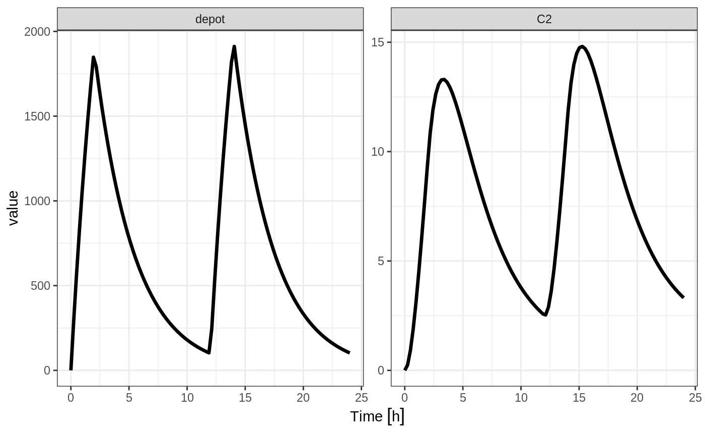
Similarly, you may also model rate. This is equivalent to NONMEM’s rate=-1 and is how RxODE’s event table specifies the data item as well. You can also use rate=model as a mnemonic:
ev <- et(timeUnits="hr") %>%
    et(amt=10000, ii=12,until=24, rate=model) %>%
    et(seq(0, 24, length.out=100))

ev
#> -------------------------- EventTable with 101 records -------------------------
#> 1 dosing records (see x$get.dosing(); add with add.dosing or et)
#> 100 observation times (see x$get.sampling(); add with add.sampling or et)
#> multiple doses in `addl` columns, expand with x$expand(); or etExpand(x)
#> -- First part of x: ------------------------------------------------------------
#> # A tibble: 101 x 6
#> time amt rate ii addl evid
#> [h] <dbl> <rate/dur> [h] <int> <evid>
#> 1 0.0000000 NA NA NA NA 0:Observation
#> 2 0.0000000 10000 -1:rate 12 2 1:Dose (Add)
#> 3 0.2424242 NA NA NA NA 0:Observation
#> 4 0.4848485 NA NA NA NA 0:Observation
#> 5 0.7272727 NA NA NA NA 0:Observation
#> 6 0.9696970 NA NA NA NA 0:Observation
#> 7 1.2121212 NA NA NA NA 0:Observation
#> 8 1.4545455 NA NA NA NA 0:Observation
#> 9 1.6969697 NA NA NA NA 0:Observation
#> 10 1.9393939 NA NA NA NA 0:Observation
#> # ... with 91 more rows
#> --------------------------------------------------------------------------------
Steady State
Steady state doses; These doses are solved until a steady state is reached with a constant inter-dose interval.
#> -------------------------- EventTable with 101 records -------------------------
#>    1 dosing records (see x$get.dosing(); add with add.dosing or et)
#>    100 observation times (see x$get.sampling(); add with add.sampling or et)
#> -- First part of x: ------------------------------------------------------------
#> # A tibble: 101 x 5
#>         time   amt    ii evid             ss
#>          [h] <dbl>   [h] <evid>        <int>
#>  1 0.0000000    NA    NA 0:Observation    NA
#>  2 0.0000000 10000    12 1:Dose (Add)      1
#>  3 0.2424242    NA    NA 0:Observation    NA
#>  4 0.4848485    NA    NA 0:Observation    NA
#>  5 0.7272727    NA    NA 0:Observation    NA
#>  6 0.9696970    NA    NA 0:Observation    NA
#>  7 1.2121212    NA    NA 0:Observation    NA
#>  8 1.4545455    NA    NA 0:Observation    NA
#>  9 1.6969697    NA    NA 0:Observation    NA
#> 10 1.9393939    NA    NA 0:Observation    NA
#> # ... with 91 more rows
#> --------------------------------------------------------------------------------
Steady state for complex dosing
By using the ss=2 flag, you can use the super-positioning principle in linear kinetics to get steady state nonstandard dosing (i.e. morning 100 mg vs evening 150 mg). This is done by:
- Saving all the state values
- Resetting all the states and solving the system to steady state
- Adding back all the prior state values
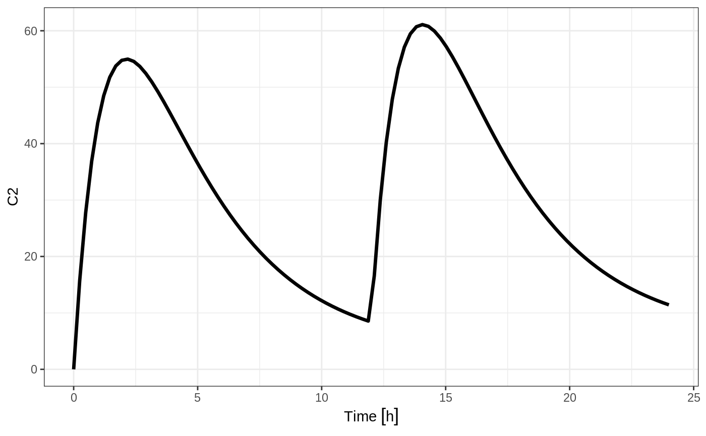
ev <- et(timeUnits="hr") %>%
    et(amt=10000, ii=24, ss=1) %>%
    et(time=12, amt=15000, ii=24, ss=2) %>%
    et(time=24, amt=10000, ii=24, addl=3) %>%
    et(time=36, amt=15000, ii=24, addl=3) %>%
    et(seq(0, 64, length.out=500))

library(ggplot2)

rxSolve(m1, ev,maxsteps=10000) %>% plot(C2) +
    annotate("rect", xmin=0, xmax=24, ymin=-Inf, ymax=Inf, alpha=0.2) +
    annotate("text", x=12.5, y=7, label="Initial Steady State Period") +
    annotate("text", x=44,   y=7, label="Steady State AM/PM dosing")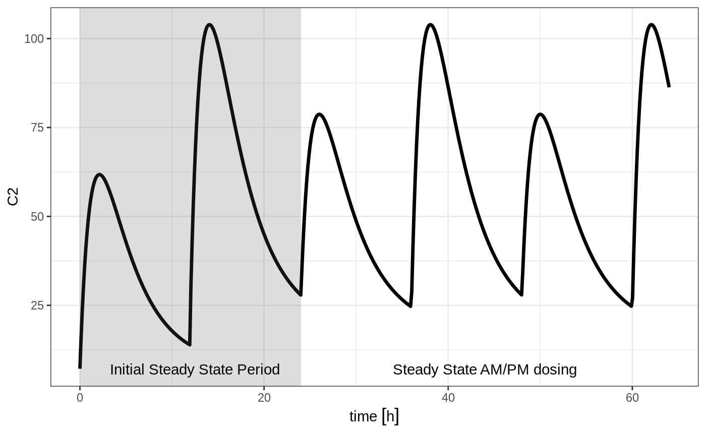
You can see that it takes a full dose cycle to reach the true complex steady state dosing.
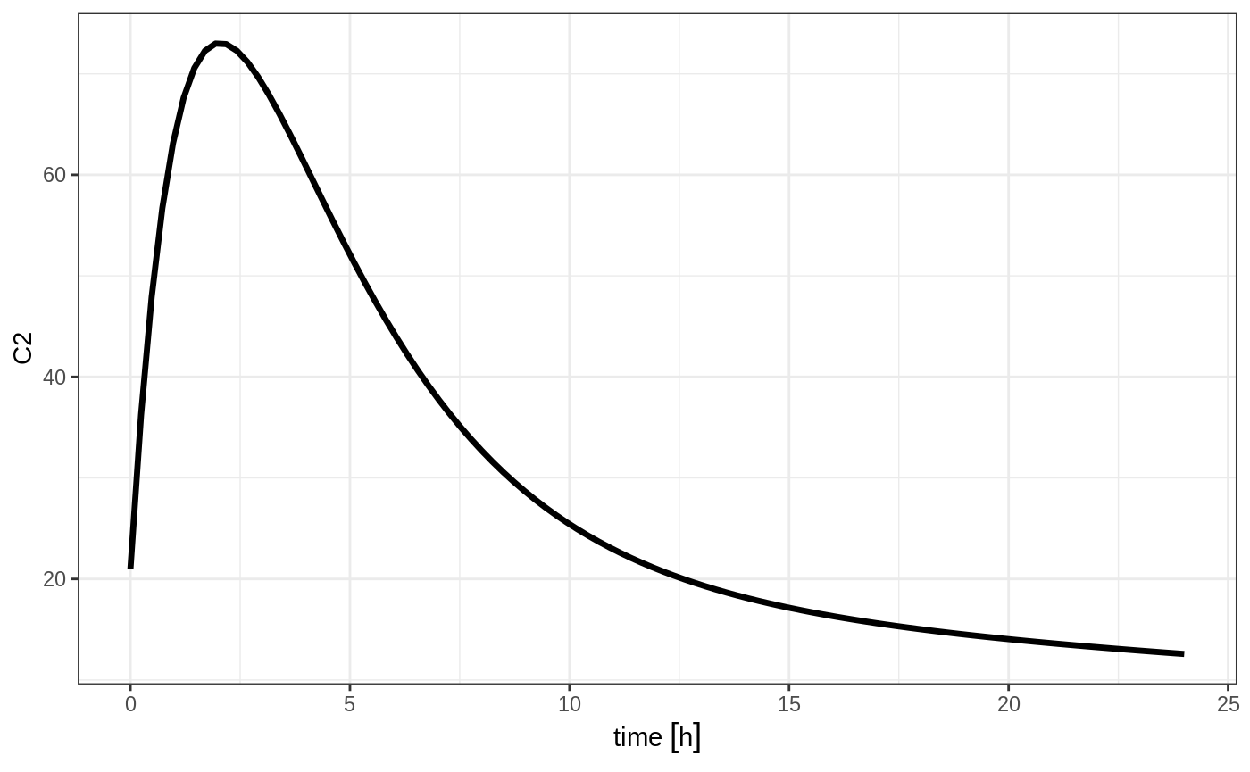
Steady state for constant infusion or zero order processes
The last type of steady state that RxODE supports is steady-state constant infusion rate. This can be specified the same way as NONMEM, that is:
- No inter-dose interval
ii=0 - A steady state dose, ie
ss=1 - Either a positive rate (
rate>0) or a estimated raterate=-1. - A zero dose, ie
amt=0 - Once the steady-state constant infusion is achieved, the infusion is turned off when using this record, just like NONMEM.
Note that rate=-2 where we model the duration of infusion doesn’t make much sense since we are solving the infusion until steady state. The duration is specified by the steady state solution.
Also note that bioavailability changes on this steady state infusion also do not make sense because they neither change the rate or the duration of the steady state infusion. Hence modeled bioavailability on this type of dosing event is ignored.
Here is an example:
ev <- et(timeUnits="hr") %>%
    et(amt=0, ss=1,rate=10000/8)

p1 <- rxSolve(m1, ev) %>% plot(C2, eff)


ev <- et(timeUnits="hr") %>%
    et(amt=200000, rate=10000/8) %>%
    et(0, 250, length.out=1000)

p2 <- rxSolve(m1, ev) %>% plot(C2, eff)


grid.arrange(p1,p2, ncol=1)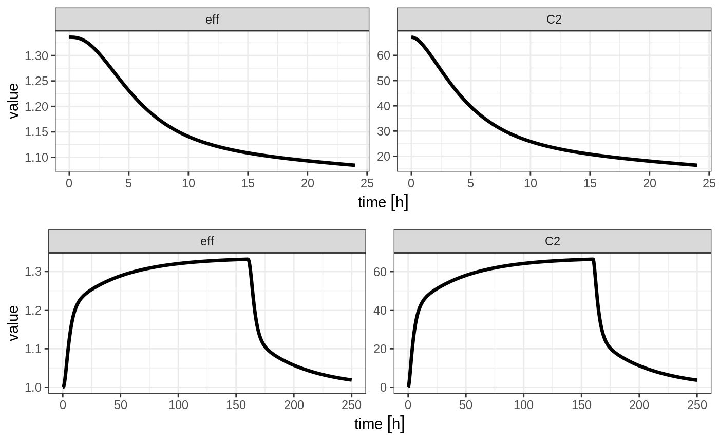
Not only can this be used for PK, it can be used for steady-state disease processes.
Reset Events
Reset events are implemented by evid=3 or evid=reset, for reset and evid=4 for reset and dose.
ev <- et(timeUnits="hr") %>%
    et(amt=10000, ii=12, addl=3) %>%
    et(time=6, evid=reset) %>%
    et(seq(0, 24, length.out=100))

ev
#> -------------------------- EventTable with 102 records -------------------------
#> 2 dosing records (see x$get.dosing(); add with add.dosing or et)
#> 100 observation times (see x$get.sampling(); add with add.sampling or et)
#> multiple doses in `addl` columns, expand with x$expand(); or etExpand(x)
#> -- First part of x: ------------------------------------------------------------
#> # A tibble: 102 x 5
#> time amt ii addl evid
#> [h] <dbl> [h] <int> <evid>
#> 1 0.0000000 NA NA NA 0:Observation
#> 2 0.0000000 10000 12 3 1:Dose (Add)
#> 3 0.2424242 NA NA NA 0:Observation
#> 4 0.4848485 NA NA NA 0:Observation
#> 5 0.7272727 NA NA NA 0:Observation
#> 6 0.9696970 NA NA NA 0:Observation
#> 7 1.2121212 NA NA NA 0:Observation
#> 8 1.4545455 NA NA NA 0:Observation
#> 9 1.6969697 NA NA NA 0:Observation
#> 10 1.9393939 NA NA NA 0:Observation
#> # ... with 92 more rows
#> --------------------------------------------------------------------------------The solving show what happens in this system when the system is reset at 6 hours post-dose.
You can see all the compartments are reset to their initial values. The next dose start the dosing cycle over.
ev <- et(timeUnits="hr") %>%
    et(amt=10000, ii=12, addl=3) %>%
    et(time=6, amt=10000, evid=4) %>%
    et(seq(0, 24, length.out=100))

ev
#> -------------------------- EventTable with 102 records -------------------------
#> 2 dosing records (see x$get.dosing(); add with add.dosing or et)
#> 100 observation times (see x$get.sampling(); add with add.sampling or et)
#> multiple doses in `addl` columns, expand with x$expand(); or etExpand(x)
#> -- First part of x: ------------------------------------------------------------
#> # A tibble: 102 x 5
#> time amt ii addl evid
#> [h] <dbl> [h] <int> <evid>
#> 1 0.0000000 NA NA NA 0:Observation
#> 2 0.0000000 10000 12 3 1:Dose (Add)
#> 3 0.2424242 NA NA NA 0:Observation
#> 4 0.4848485 NA NA NA 0:Observation
#> 5 0.7272727 NA NA NA 0:Observation
#> 6 0.9696970 NA NA NA 0:Observation
#> 7 1.2121212 NA NA NA 0:Observation
#> 8 1.4545455 NA NA NA 0:Observation
#> 9 1.6969697 NA NA NA 0:Observation
#> 10 1.9393939 NA NA NA 0:Observation
#> # ... with 92 more rows
#> --------------------------------------------------------------------------------In this case, the whole system is reset and the dose is given
Turning off compartments
You may also turn off a compartment, which is similar to a reset event.
ev <- et(timeUnits="hr") %>%
    et(amt=10000, ii=12, addl=3) %>%
    et(time=6, cmt="-depot", evid=2) %>%
    et(seq(0, 24, length.out=100))

ev
#> -------------------------- EventTable with 102 records -------------------------
#> 2 dosing records (see x$get.dosing(); add with add.dosing or et)
#> 100 observation times (see x$get.sampling(); add with add.sampling or et)
#> multiple doses in `addl` columns, expand with x$expand(); or etExpand(x)
#> -- First part of x: ------------------------------------------------------------
#> # A tibble: 102 x 6
#> time cmt amt ii addl evid
#> [h] <chr> <dbl> [h] <int> <evid>
#> 1 0.0000000 (obs) NA NA NA 0:Observation
#> 2 0.0000000 (default) 10000 12 3 1:Dose (Add)
#> 3 0.2424242 (obs) NA NA NA 0:Observation
#> 4 0.4848485 (obs) NA NA NA 0:Observation
#> 5 0.7272727 (obs) NA NA NA 0:Observation
#> 6 0.9696970 (obs) NA NA NA 0:Observation
#> 7 1.2121212 (obs) NA NA NA 0:Observation
#> 8 1.4545455 (obs) NA NA NA 0:Observation
#> 9 1.6969697 (obs) NA NA NA 0:Observation
#> 10 1.9393939 (obs) NA NA NA 0:Observation
#> # ... with 92 more rows
#> --------------------------------------------------------------------------------Solving shows what this does in the system:
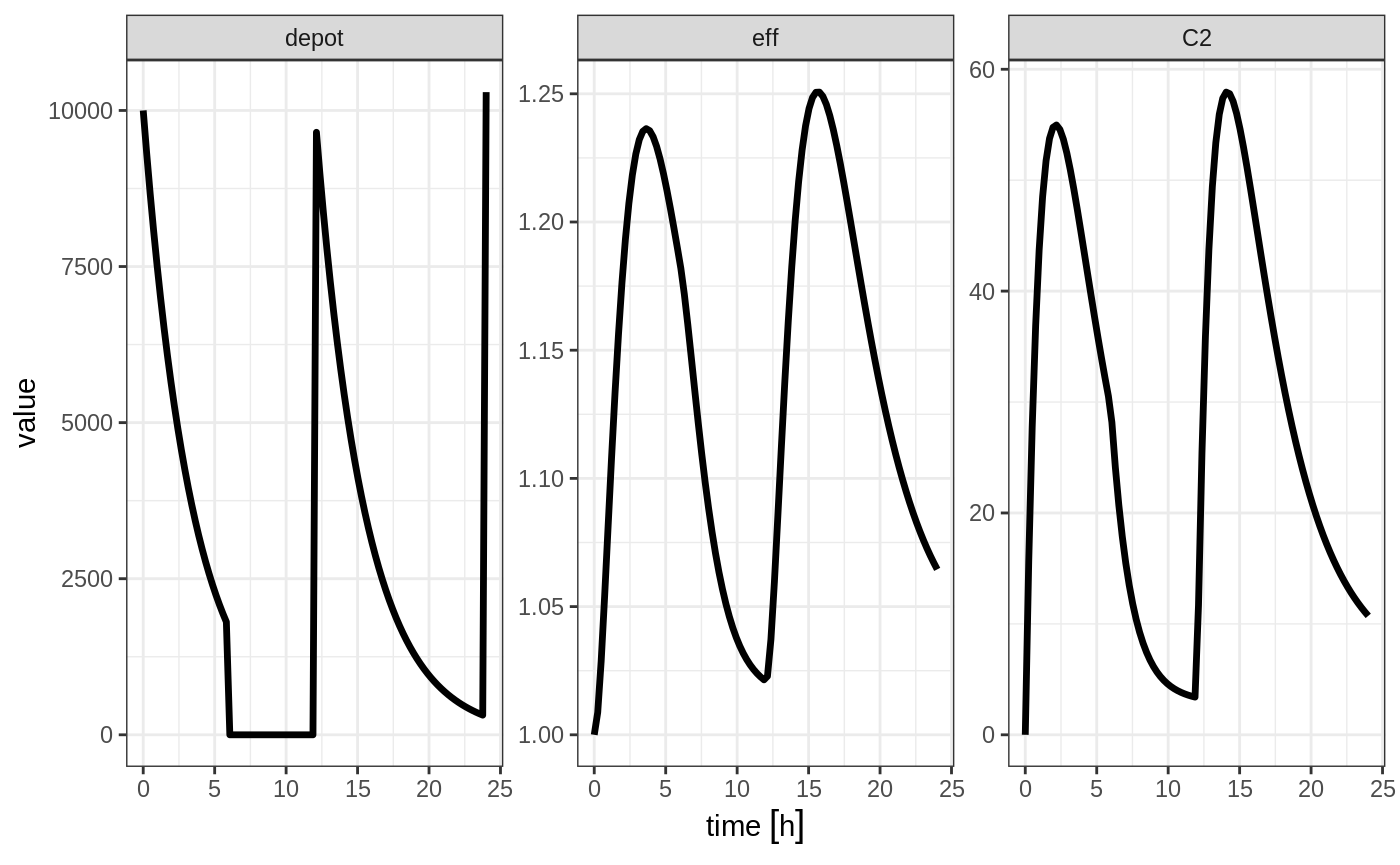
In this case, the depot is turned off, and the compartment concentrations are set to the initial values but the other compartment concentrations/levels are not reset. When another dose to the depot is administered the depot compartment is turned back on.
Note that a dose to a compartment only turns back on the compartment that was dosed. Hence if you turn off the effect compartment, it continues to be off after another dose to the depot.
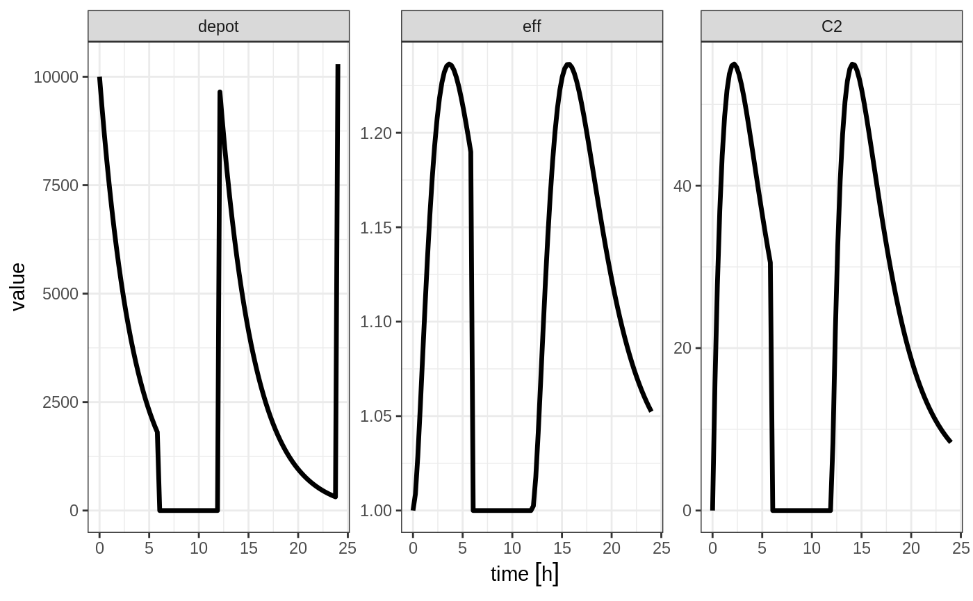
ev <- et(timeUnits="hr") %>%
    et(amt=10000, ii=12, addl=3) %>%
    et(time=6, cmt="-eff", evid=2) %>%
    et(seq(0, 24, length.out=100))

rxSolve(m1, ev) %>% plot(depot,C2, eff)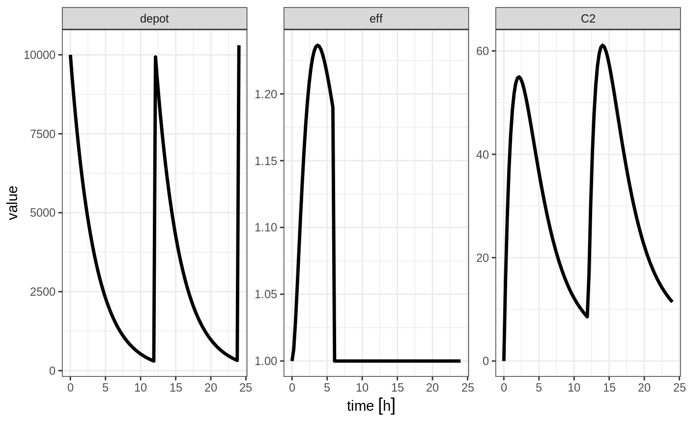
To turn back on the compartment, a zero-dose to the compartment or a evid=2 with the compartment would be needed.
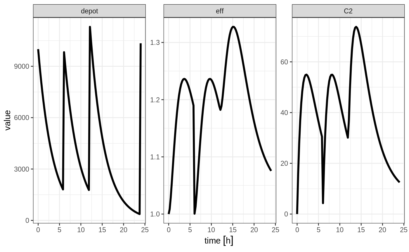
ev <- et(timeUnits="hr") %>%
    et(amt=10000, ii=12, addl=3) %>%
    et(time=6, cmt="-eff", evid=2) %>%
    et(time=12,cmt="eff",evid=2) %>%
    et(seq(0, 24, length.out=100))

rxSolve(m1, ev) %>% plot(depot,C2, eff)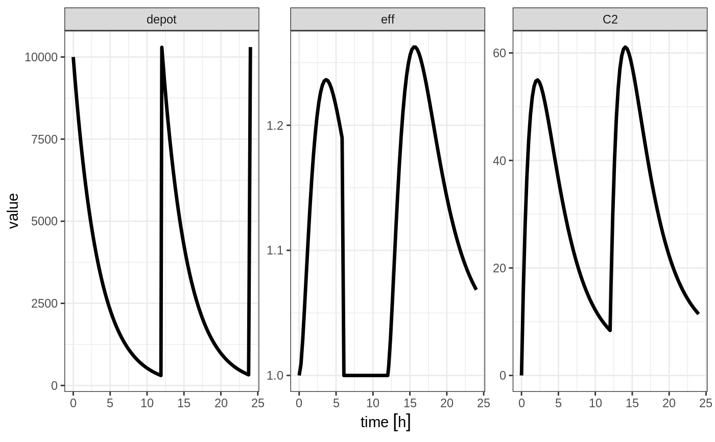
Classic RxODE evid values
While RxODE still supports these values, this is primarily provided for historic information, and we recommend using the normal NONMEM dataset standard that is used by many modeling tools like NONMEM, Monolix and nlmixr, described above.
Classically, RxODE supported event coding in a single event id evid described in the following table.
| 100+ cmt | Infusion/Event Flag | <99 Cmt | SS flag & Turning of Compartment |
|---|---|---|---|
| 100+ cmt | 0 = bolus dose | < 99 cmt | 1 = dose |
| 1 = infusion (rate) | 10 = Steady state 1 (equivalent to SS=1) | ||
| 2 = infusion (dur) | 20 = Steady state 2 (equivalent to SS=2) | ||
| 6 = turn off modeled duration | 30 = Turn off a compartment (equivalent to -CMT w/EVID=2) | ||
| 7 = turn off modeled rate | |||
| 8 = turn on modeled duration | |||
| 9 = turn on modeled rate | |||
| 4 = replace event | |||
| 5 = multiply event |
The classic EVID concatenate the numbers in the above table, so an infusion would to compartment 1 would be 10101 and an infusion to compartment 199 would be 119901.
EVID = 0 (observations), EVID=2 (other type event) and EVID=3 are all supported. Internally an EVID=9 is a non-observation event and makes sure the system is initialized to zero; EVID=9 should not be manually set. EVID 10-99 represents modeled time interventions, similar to NONMEM’s MTIME. This along with amount (amt) and time columns specify the events in the ODE system.
For infusions specified with EVIDs > 100 the amt column represents the rate value.
For Infusion flags 1 and 2 +amt turn on the infusion to a specific compartment -amt turn off the infusion to a specific compartment. To specify a dose/duration you place the dosing records at the time the duration starts or stops.
For modeled rate/duration infusion flags the on infusion flag must be followed by an off infusion record.
These number are concatenated together to form a full RxODE event ID, as shown in the following examples:
Bolus Dose Examples
A 100 bolus dose to compartment #1 at time 0
| time | evid | amt |
|---|---|---|
| 0 | 101 | 100 |
| 0.5 | 0 | 0 |
| 1 | 0 | 0 |
A 100 bolus dose to compartment #99 at time 0
| time | evid | amt |
|---|---|---|
| 0 | 9901 | 100 |
| 0.5 | 0 | 0 |
| 1 | 0 | 0 |
A 100 bolus dose to compartment #199 at time 0
| time | evid | amt |
|---|---|---|
| 0 | 109901 | 100 |
| 0.5 | 0 | 0 |
| 1 | 0 | 0 |
Infusion Event Examples
Bolus infusion with rate 50 to compartment 1 for 1.5 hr, (modeled bioavailability changes duration of infusion)
| time | evid | amt |
|---|---|---|
| 0 | 10101 | 50 |
| 0.5 | 0 | 0 |
| 1 | 0 | 0 |
| 1.5 | 10101 | -50 |
Bolus infusion with rate 50 to compartment 1 for 1.5 hr (modeled bioavailability changes rate of infusion)
| time | evid | amt |
|---|---|---|
| 0 | 20101 | 50 |
| 0.5 | 0 | 0 |
| 1 | 0 | 0 |
| 1.5 | 20101 | -50 |
Modeled rate with amount of 50
| time | evid | amt |
|---|---|---|
| 0 | 90101 | 50 |
| 0 | 70101 | 50 |
| 0.5 | 0 | 0 |
| 1 | 0 | 0 |
Modeled duration with amount of 50
| time | evid | amt |
|---|---|---|
| 0 | 80101 | 50 |
| 0 | 60101 | 50 |
| 0.5 | 0 | 0 |
| 1 | 0 | 0 |
Steady State for classic RxODE EVID example
Steady state dose to cmt 1
| time | evid | amt |
|---|---|---|
| 0 | 110 | 50 |
Steady State with super-positioning principle for am 50 and pm 100 dose
| time | evid | amt |
|---|---|---|
| 0 | 110 | 50 |
| 12 | 120 | 100 |
Turning off a compartment with classic RxODE EVID
Turn off the first compartment at time 12
| time | evid | amt |
|---|---|---|
| 0 | 110 | 50 |
| 12 | 130 | NA |
Event coding in RxODE is encoded in a single event number evid. For compartments under 100, this is coded as:
- This event is
0for observation events. - For a specified compartment a bolus dose is defined as:
- 100*(Compartment Number) + 1
- The dose is then captured in the
amt - For IV bolus doses the event is defined as:
- 10000 + 100*(Compartment Number) + 1
- The infusion rate is captured in the
amtcolumn - The infusion is turned off by subtracting
amtwith the sameevidat the stop of the infusion.
For compartments greater or equal to 100, the 100s place and above digits are transferred to the 100,000th place digit. For doses to the 99th compartment the evid for a bolus dose would be 9901 and the evid for an infusion would be 19901. For a bolus dose to the 199th compartment the evid for the bolus dose would be 109901. An infusion dosing record for the 199th compartment would be 119901.