Speeding up RxODE
Matthew Fidler
2019-10-16
RxODE-speed.RmdIncreasing RxODE speed by multi-subject parallel solving
RxODE originally developed as an ODE solver that allowed an ODE solve for a single subject. This flexibility is still supported.
The original code from the RxODE tutorial is below:
library(RxODE)
library(microbenchmark)
library(mvnfast)

mod1 <- RxODE({
    C2 = centr/V2;
    C3 = peri/V3;
    d/dt(depot) = -KA*depot;
    d/dt(centr) = KA*depot - CL*C2 - Q*C2 + Q*C3;
    d/dt(peri) = Q*C2 - Q*C3;
    d/dt(eff) = Kin - Kout*(1-C2/(EC50+C2))*eff;
    eff(0) = 1
})

## Create an event table

ev <- et() %>%
    et(amt=10000, addl=9,ii=12) %>%
    et(time=120, amt=20000, addl=4, ii=24) %>%
    et(0:240) ## Add Sampling

nsub <- 100 # 100 subproblems
sigma <- matrix(c(0.09,0.08,0.08,0.25),2,2) # IIV covariance matrix
mv <- rmvn(n=nsub, rep(0,2), sigma) # Sample from covariance matrix
CL <- 7*exp(mv[,1])
V2 <- 40*exp(mv[,2])
params.all <- cbind(KA=0.3, CL=CL, V2=V2, Q=10, V3=300,
                    Kin=0.2, Kout=0.2, EC50=8)
For Loop
The slowest way to code this is to use a for loop. In this example we will enclose it in a function to compare timing.
Running with apply
In general for R, the apply types of functions perform better than a for loop, so the tutorial also suggests this speed enhancement
runSapply <- function(){
    res <- apply(params.all, 1, function(theta)
        mod1$run(theta, ev)[, "eff"])
}
Run using a single-threaded solve
You can also have RxODE solve all the subject simultaneously without collecting the results in R, using a single threaded solve.
The data output is slightly different here, but still gives the same information:
Run a 2 threaded solve
RxODE supports multi-threaded solves, so another option is to have 2 threads (called cores in the solve options, you can see the options in rxControl() or rxSolve()).
Compare the times between all the methods
Now the moment of truth, the timings:
bench <- microbenchmark(runFor(), runSapply(), runSingleThread(),run2Thread())
print(bench)
#> Unit: milliseconds
#>               expr        min         lq       mean     median         uq
#>           runFor() 2459.97537 3101.80238 3235.83700 3249.87800 3426.61862
#>        runSapply() 2466.99591 3081.91888 3215.02331 3202.05876 3364.09040
#>  runSingleThread()   31.12156   43.26954   57.11588   52.34140   71.89627
#>       run2Thread()   17.08877   28.56109   36.36301   34.20892   44.62769
#>         max neval
#>  3922.26266   100
#>  3996.17092   100
#>    95.28235   100
#> 63.12042 100plot(bench)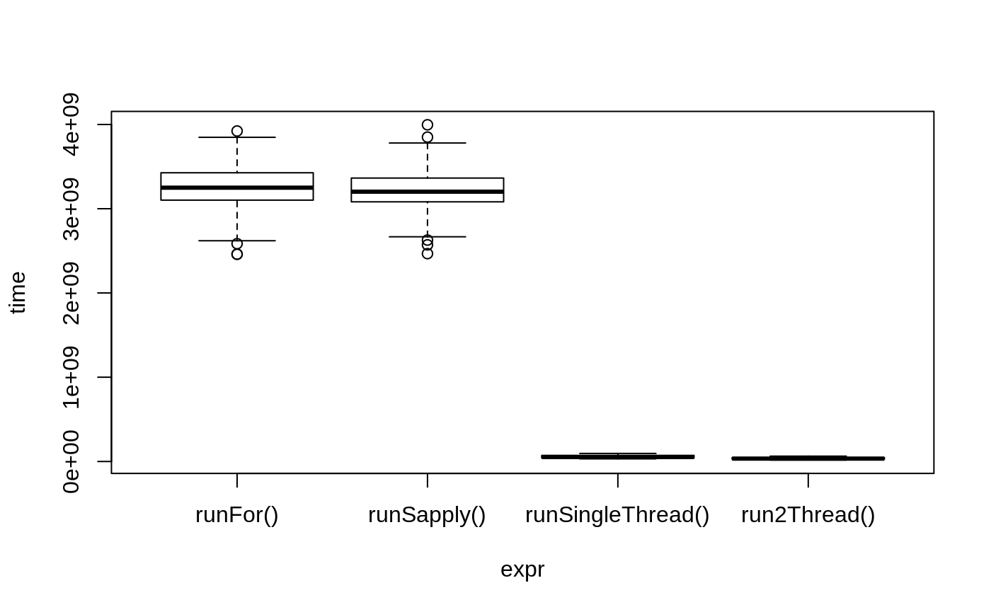
It is clear that the largest jump in performance when using the solve method and providing all the parameters to RxODE to solve without looping over each subject with either a for or a sapply. The number of cores/threads applied to the solve also plays a role in the solving.
We can explore the number of threads further with the following code:
runThread <- function(n){
    solve(mod1, params.all, ev, cores=n)[,c("sim.id", "time", "eff")]
}

bench <- eval(parse(text=sprintf("microbenchmark(%s)",
                                     paste(paste0("runThread(", seq(1, rxCores()),")"),
                                           collapse=","))))
print(bench)
#> Unit: milliseconds
#>           expr      min       lq     mean   median       uq      max neval
#>   runThread(1) 29.91025 32.51644 34.22549 33.89869 35.49776 54.40221   100
#>   runThread(2) 16.37059 17.80370 21.89147 18.53547 26.02539 44.69197   100
#>   runThread(3) 12.22658 13.29381 17.52575 13.87890 21.53759 34.59217   100
#>   runThread(4) 10.11942 11.08054 15.30856 14.99501 17.80574 31.75803   100
#>   runThread(5) 13.72407 14.75192 16.75424 15.30397 16.61651 25.49704   100
#>   runThread(6) 12.31904 13.25242 15.52834 14.15435 15.15266 24.64866   100
#>   runThread(7) 11.20890 12.49975 14.49545 13.20765 14.79877 24.23919   100
#>   runThread(8) 10.87229 11.95732 13.64890 12.58088 13.49910 23.80908   100
#>   runThread(9) 10.25690 11.64922 13.96999 12.70091 14.88986 25.00136   100
#>  runThread(10) 10.37223 12.21643 16.46894 14.97692 20.11870 32.67531   100
#>  runThread(11) 13.47055 28.96028 30.60698 31.37003 32.61970 46.90703   100
#> runThread(12) 20.12782 30.26269 32.61500 31.91789 33.96171 48.01449 100plot(bench)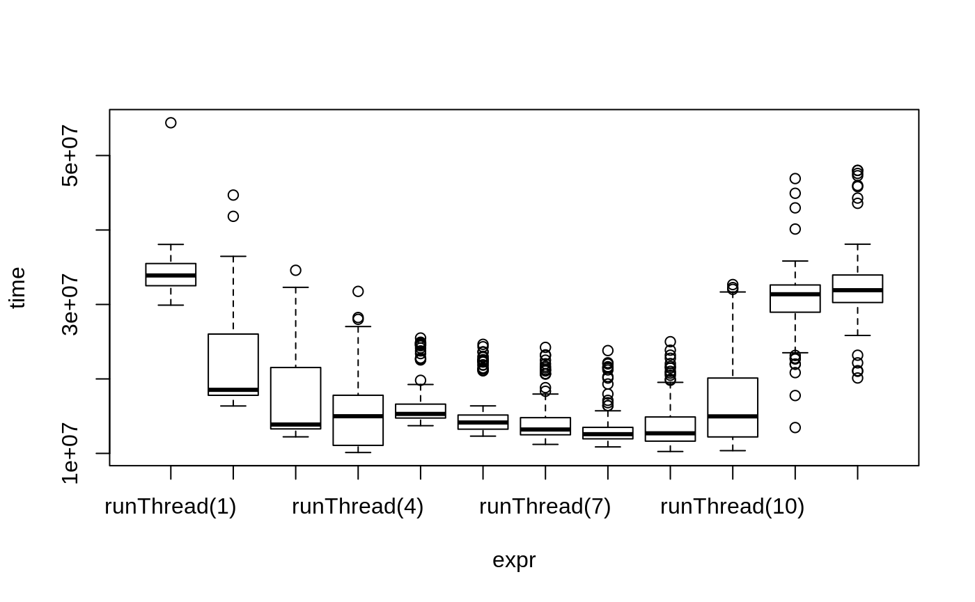
There is a suite spot in speed vs number or cores. The system type, complexity of the ODE solving and the number of subjects may affect this arbitrary number of threads. 4 threads is a good number to use without any prior knowledge because most systems these days have at least 4 threads (or 2 processors with 4 threads).
Want more ways to run multi-subject simulations
The version since the tutorial has even more ways to run multi-subject simulations, including adding variability in sampling and dosing times with et() (see RxODE events for more information), ability to supply both an omega and sigma matrix as well as adding as a thetaMat to R to simulate with uncertainty in the omega, sigma and theta matrices; see RxODE simulation vignette.
Session Information
The session information:
sessionInfo()
#> R version 3.6.0 (2019-04-26)
#> Platform: x86_64-pc-linux-gnu (64-bit)
#> Running under: Gentoo/Linux
#>
#> Matrix products: default
#> BLAS:   /usr/lib64/libblas.so.3.8.0
#> LAPACK: /usr/lib64/liblapack.so.3.8.0
#>
#> locale:
#>  [1] LC_CTYPE=en_US.utf8       LC_NUMERIC=C
#>  [3] LC_TIME=en_US.utf8        LC_COLLATE=en_US.utf8
#>  [5] LC_MONETARY=en_US.utf8    LC_MESSAGES=en_US.utf8
#>  [7] LC_PAPER=en_US.utf8       LC_NAME=C
#>  [9] LC_ADDRESS=C              LC_TELEPHONE=C
#> [11] LC_MEASUREMENT=en_US.utf8 LC_IDENTIFICATION=C
#>
#> attached base packages:
#> [1] stats     graphics  grDevices utils     datasets  methods   base
#>
#> other attached packages:
#> [1] mvnfast_0.2.5        microbenchmark_1.4-7 RxODE_0.9.1-7
#>
#> loaded via a namespace (and not attached):
#>  [1] Rcpp_1.0.2       compiler_3.6.0   pillar_1.4.2     sys_3.3
#>  [5] PreciseSums_0.3  tools_3.6.0      digest_0.6.21    evaluate_0.14
#>  [9] memoise_1.1.0    tibble_2.1.3     gtable_0.3.0     pkgconfig_2.0.3
#> [13] rlang_0.4.0      yaml_2.2.0       pkgdown_1.4.1    xfun_0.10
#> [17] stringr_1.4.0    dplyr_0.8.3      knitr_1.25       desc_1.2.0
#> [21] fs_1.3.1         rprojroot_1.3-2  grid_3.6.0       tidyselect_0.2.5
#> [25] glue_1.3.1       R6_2.4.0         rmarkdown_1.16   polyclip_1.10-0
#> [29] dparser_1.3.1-0  farver_1.1.0     tweenr_1.0.1     ggplot2_3.2.1
#> [33] purrr_0.3.2      magrittr_1.5     units_0.6-5      backports_1.1.5
#> [37] scales_1.0.0     htmltools_0.4.0  MASS_7.3-51.4    assertthat_0.2.1
#> [41] mime_0.7         ggforce_0.3.1    colorspace_1.4-1 lotri_0.1.1
#> [45] stringi_1.4.3    lazyeval_0.2.2   munsell_0.5.0    markdown_1.1
#> [49] crayon_1.3.4