
library(nlmixr)
library(xpose)
#> Loading required package: ggplot2
#> 
#> Attaching package: 'xpose'
#> The following object is masked from 'package:nlmixr':
#> 
#>     vpc
#> The following object is masked from 'package:stats':
#> 
#>     filter
library(xpose.nlmixr)
#> 
#> Attaching package: 'xpose.nlmixr'
#> The following object is masked from 'package:nlmixr':
#> 
#>     vpc


wbc <- function() {
    ini({
        ## Note that the UI can take expressions
        ## Also note that these initial estimates should be provided on the log-scale
        log_CIRC0 <- log(7.21)
        log_MTT <- log(124)
        log_SLOPU <- log(28.9)
        log_GAMMA <- log(0.239)
        ## Initial estimates should be high for SAEM ETAs
        eta.CIRC0  ~ .1
        eta.MTT  ~ .03
        eta.SLOPU ~ .2
        ##  Also true for additive error (also ignored in SAEM)
        prop.err <- 10
    })
    model({
        CIRC0 =  exp(log_CIRC0 + eta.CIRC0)
        MTT =  exp(log_MTT + eta.MTT)
        SLOPU =  exp(log_SLOPU + eta.SLOPU)
        GAMMA = exp(log_GAMMA)

        # PK parameters from input dataset
        CL = CLI;
        V1 = V1I;
        V2 = V2I;
        Q = 204;

        CONC = A_centr/V1;

        # PD parameters
        NN = 3;
        KTR = (NN + 1)/MTT;
        EDRUG = 1 - SLOPU * CONC;
        FDBK = (CIRC0 / A_circ)^GAMMA;

        CIRC = A_circ;

        A_prol(0) = CIRC0;
        A_tr1(0) = CIRC0;
        A_tr2(0) = CIRC0;
        A_tr3(0) = CIRC0;
        A_circ(0) = CIRC0;

        d/dt(A_centr) = A_periph * Q/V2 - A_centr * (CL/V1 + Q/V1);
        d/dt(A_periph) = A_centr * Q/V1 - A_periph * Q/V2;
        d/dt(A_prol) = KTR * A_prol * EDRUG * FDBK - KTR * A_prol;
        d/dt(A_tr1) = KTR * A_prol - KTR * A_tr1;
        d/dt(A_tr2) = KTR * A_tr1 - KTR * A_tr2;
        d/dt(A_tr3) = KTR * A_tr2 - KTR * A_tr3;
        d/dt(A_circ) = KTR * A_tr3 - KTR * A_circ;

        CIRC ~ prop(prop.err)
    })
}

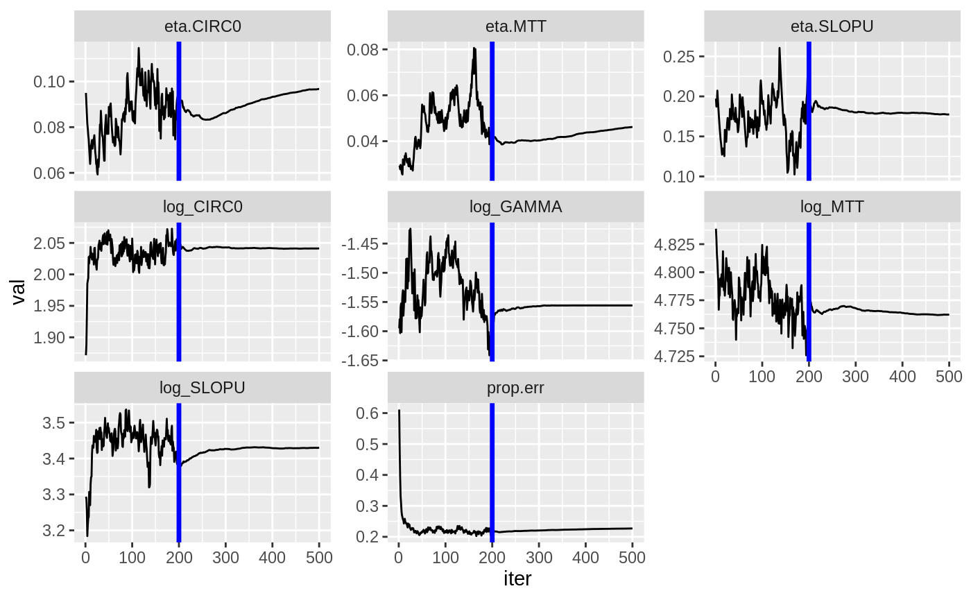
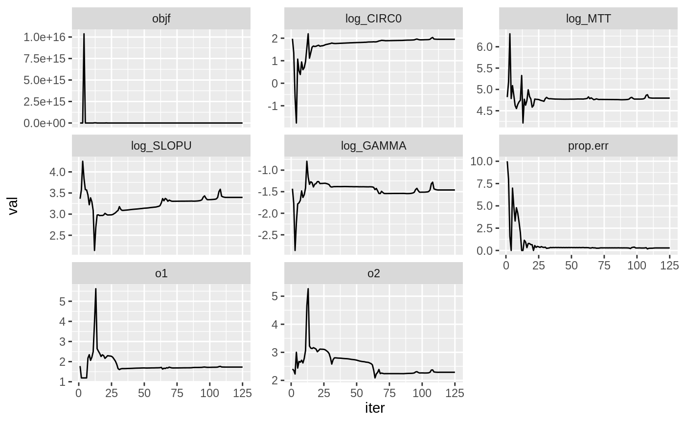
Fit model using saem

d3 = read.csv("Simulated_WBC_pacl_ddmore_samePK_nlmixr.csv", na.string = ".")

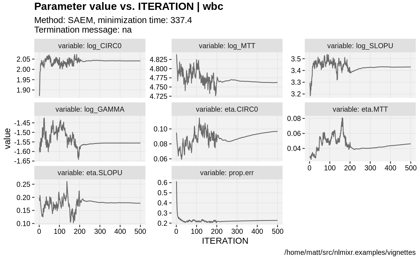
fit.S <- nlmixr(wbc, d3, est="saem", table=list(cwres=TRUE, npde=TRUE))
#> Loading model already run (/tmp/RtmpXKdUFj/temp_libpath58be457a881a/nlmixr.examples/nlmixr-wbc-d3-saem-f1f1b2aae1f74678ea021385c3b62987.rds)
#> Warning in lapply(X = X, FUN = FUN, ...): ID missing in parameters dataset;
#>  Parameters are assumed to have the same order as the IDs in the event dataset

xpdb <- xpose_data_nlmixr(fit.S)
#> Warning: `complete_()` is deprecated as of tidyr 1.0.0.
#> Please use `complete()` instead.
#> This warning is displayed once per session.
#> Call `lifecycle::last_warnings()` to see where this warning was generated.
plot(fit.S)

#> geom_path: Each group consists of only one observation. Do you need to
#> adjust the group aesthetic?
#> geom_path: Each group consists of only one observation. Do you need to
#> adjust the group aesthetic?

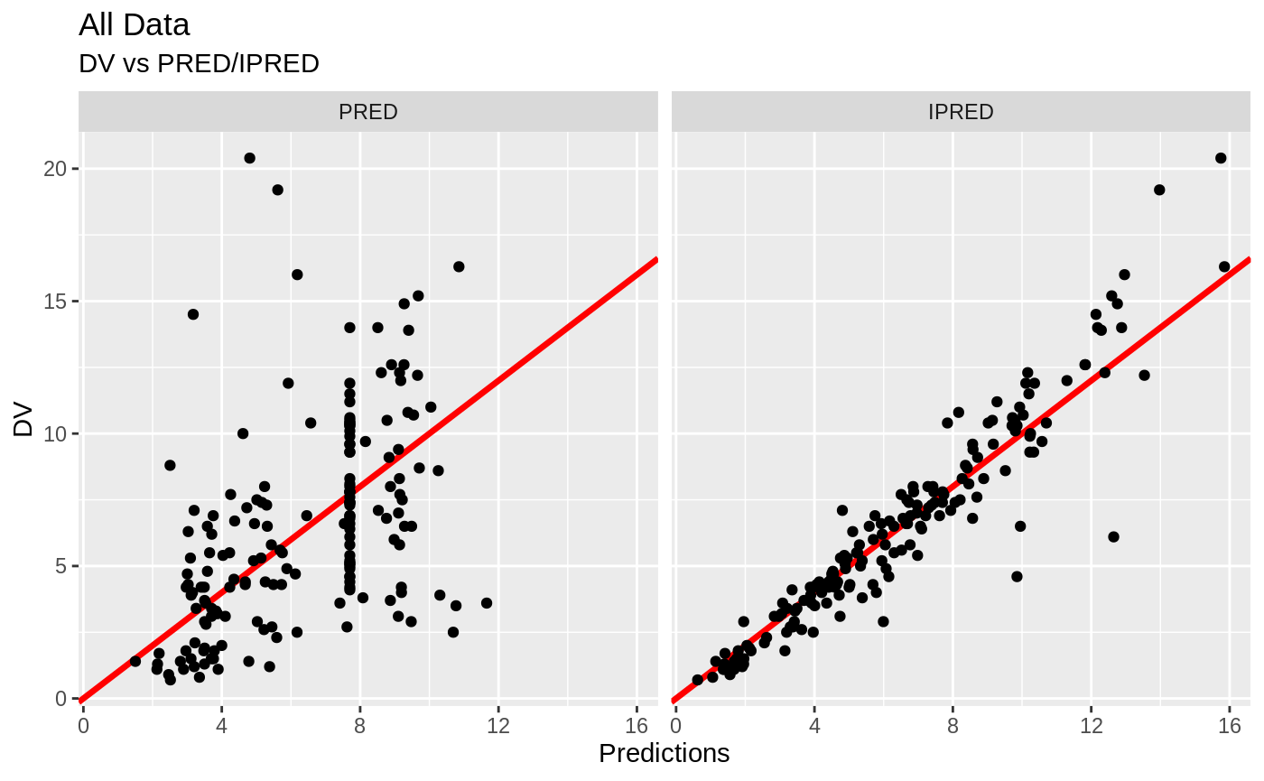
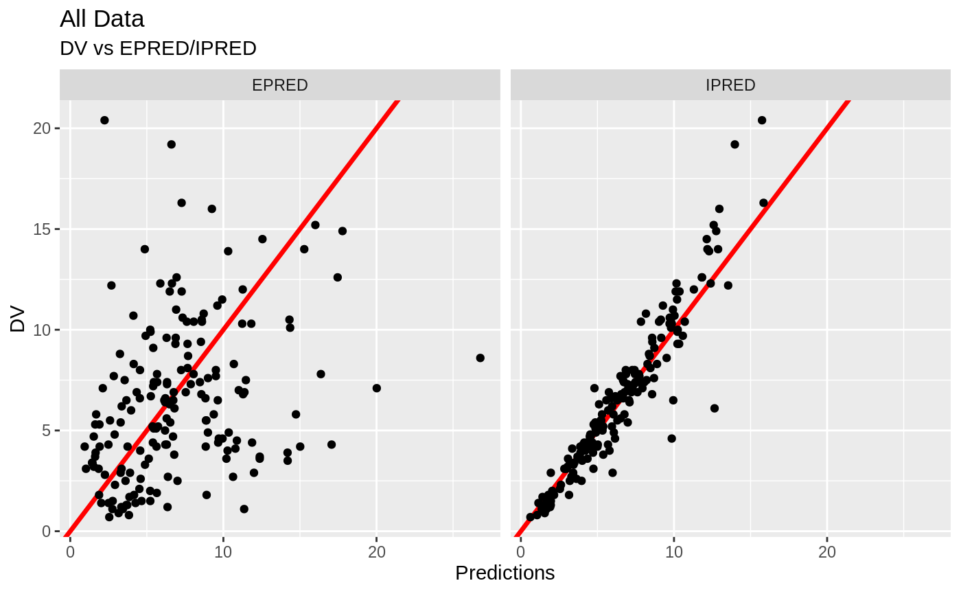
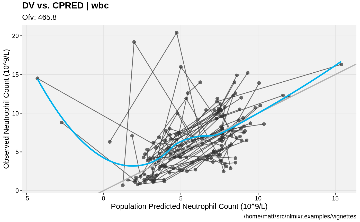
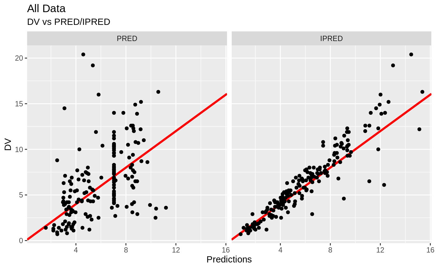
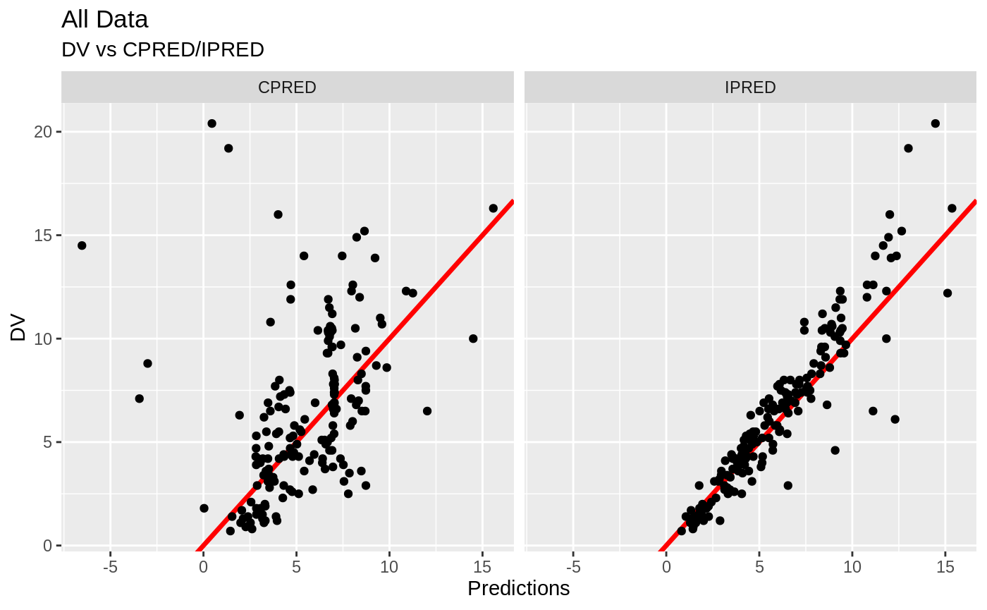
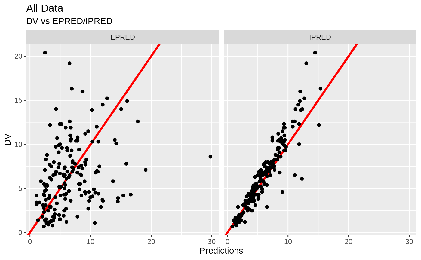
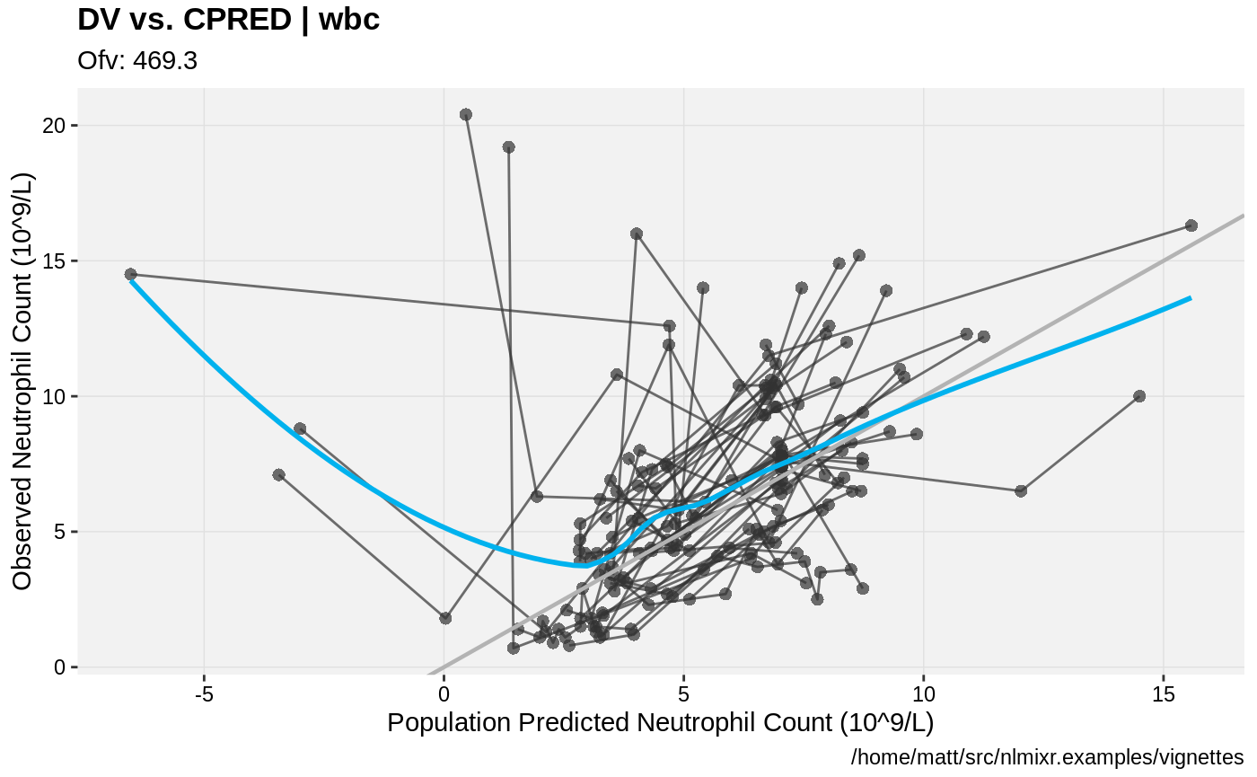
print(dv_vs_pred(xpdb) +
      ylab("Observed Neutrophil Count (10^9/L)") +
      xlab("Population Predicted Neutrophil Count (10^9/L)"))


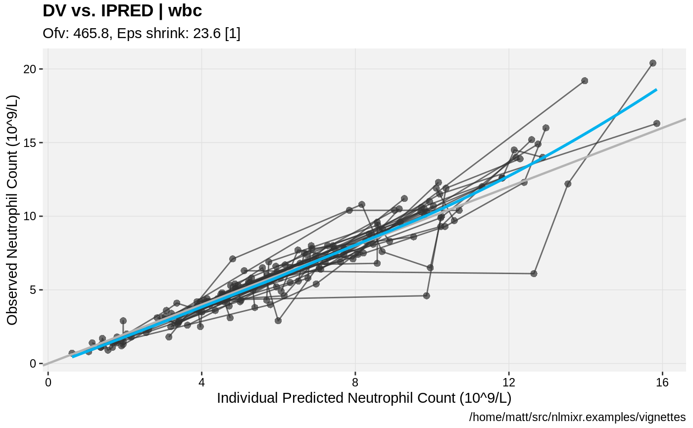
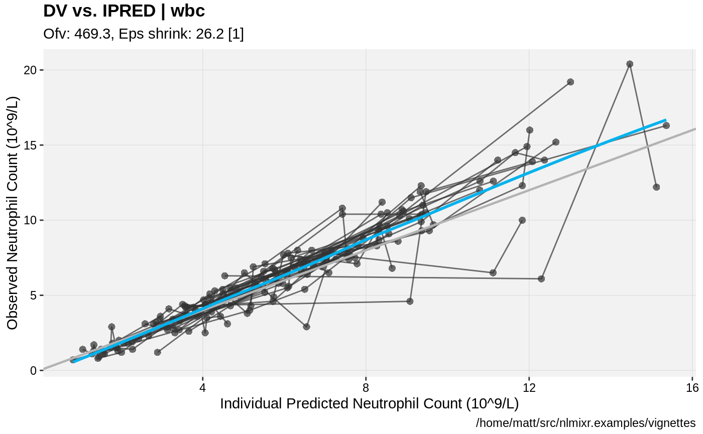
print(dv_vs_ipred(xpdb) +
      ylab("Observed Neutrophil Count (10^9/L)") +
      xlab("Individual Predicted Neutrophil Count (10^9/L)"))


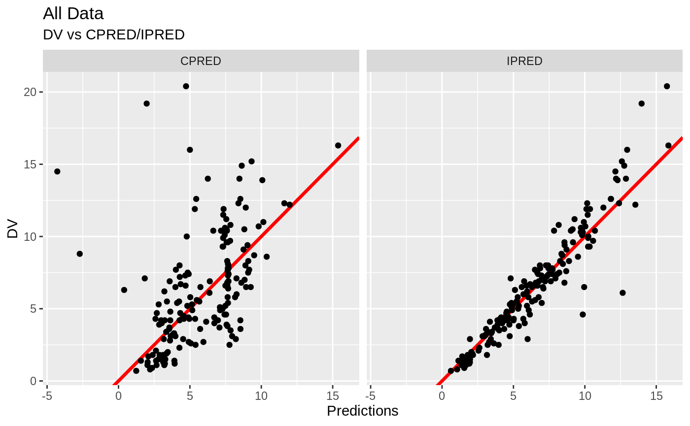
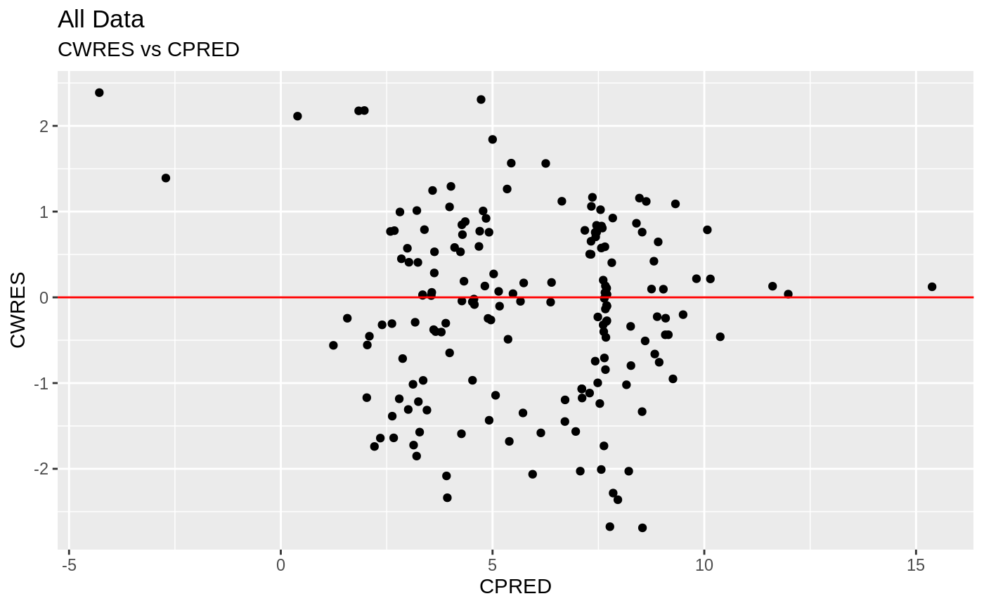
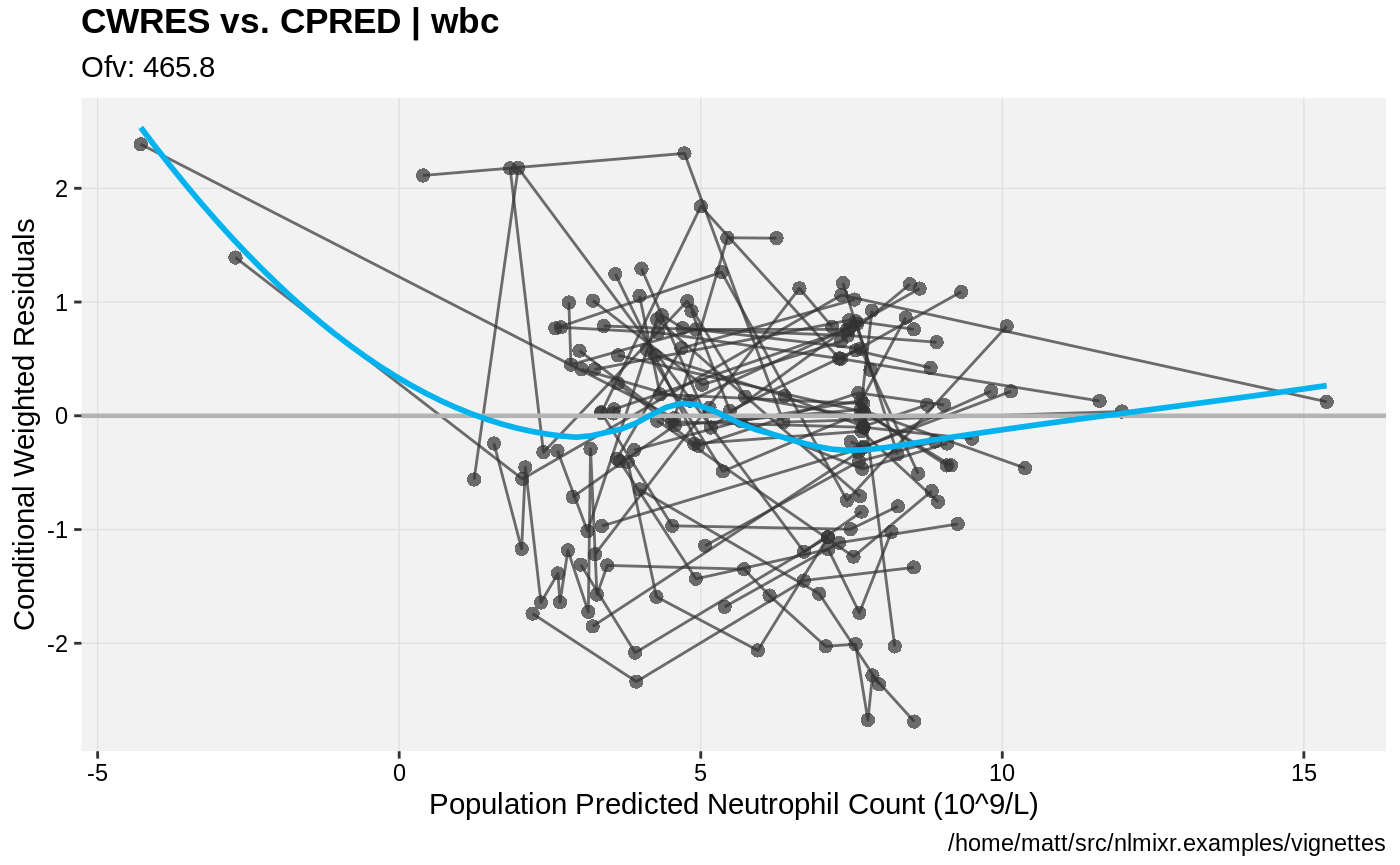
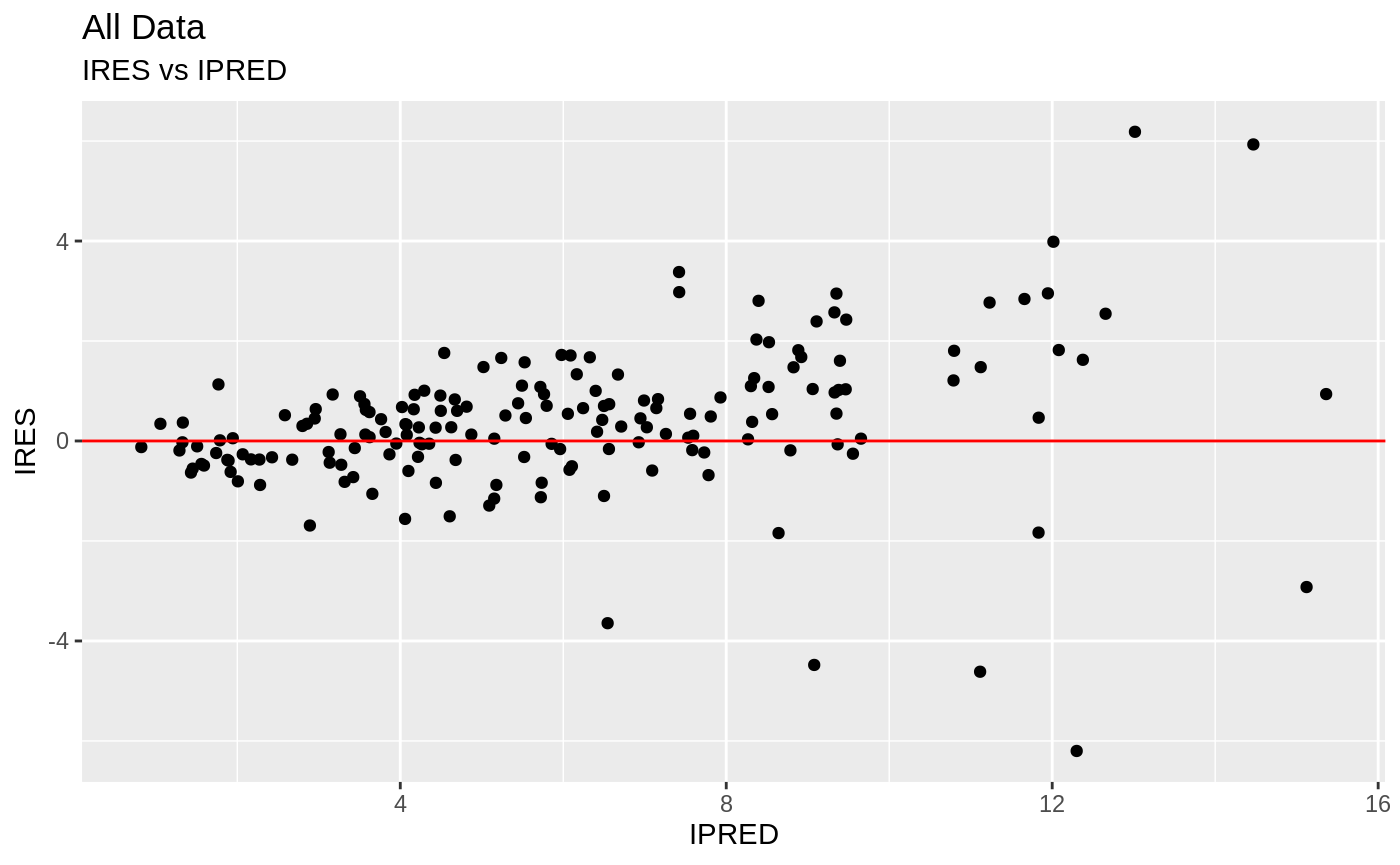
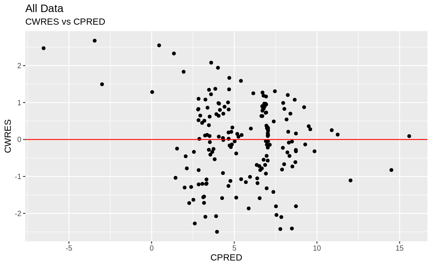
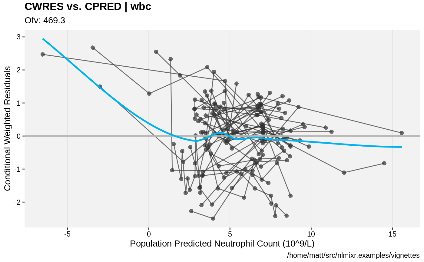
print(res_vs_pred(xpdb) +
      ylab("Conditional Weighted Residuals") +
      xlab("Population Predicted Neutrophil Count (10^9/L)"))


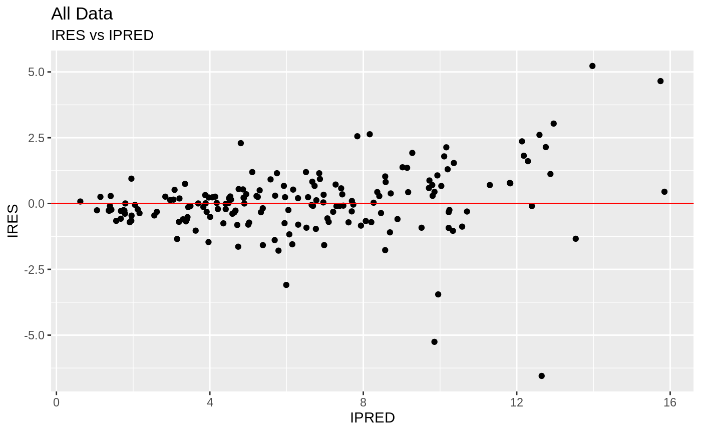
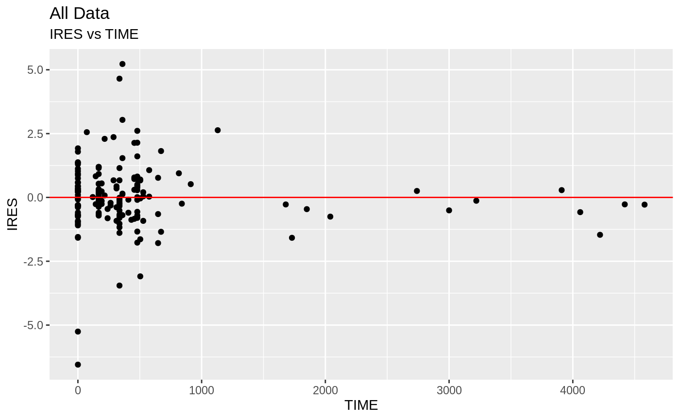
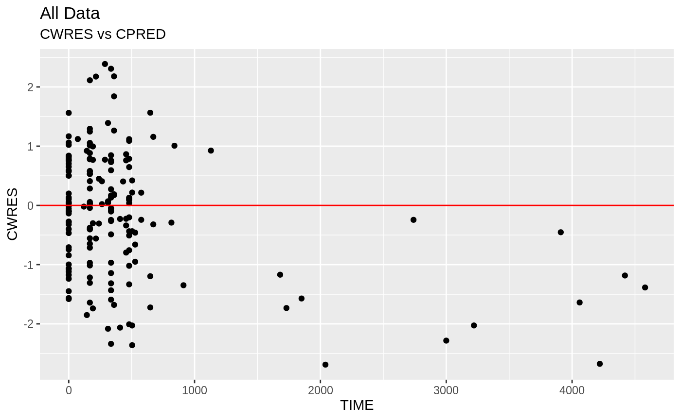
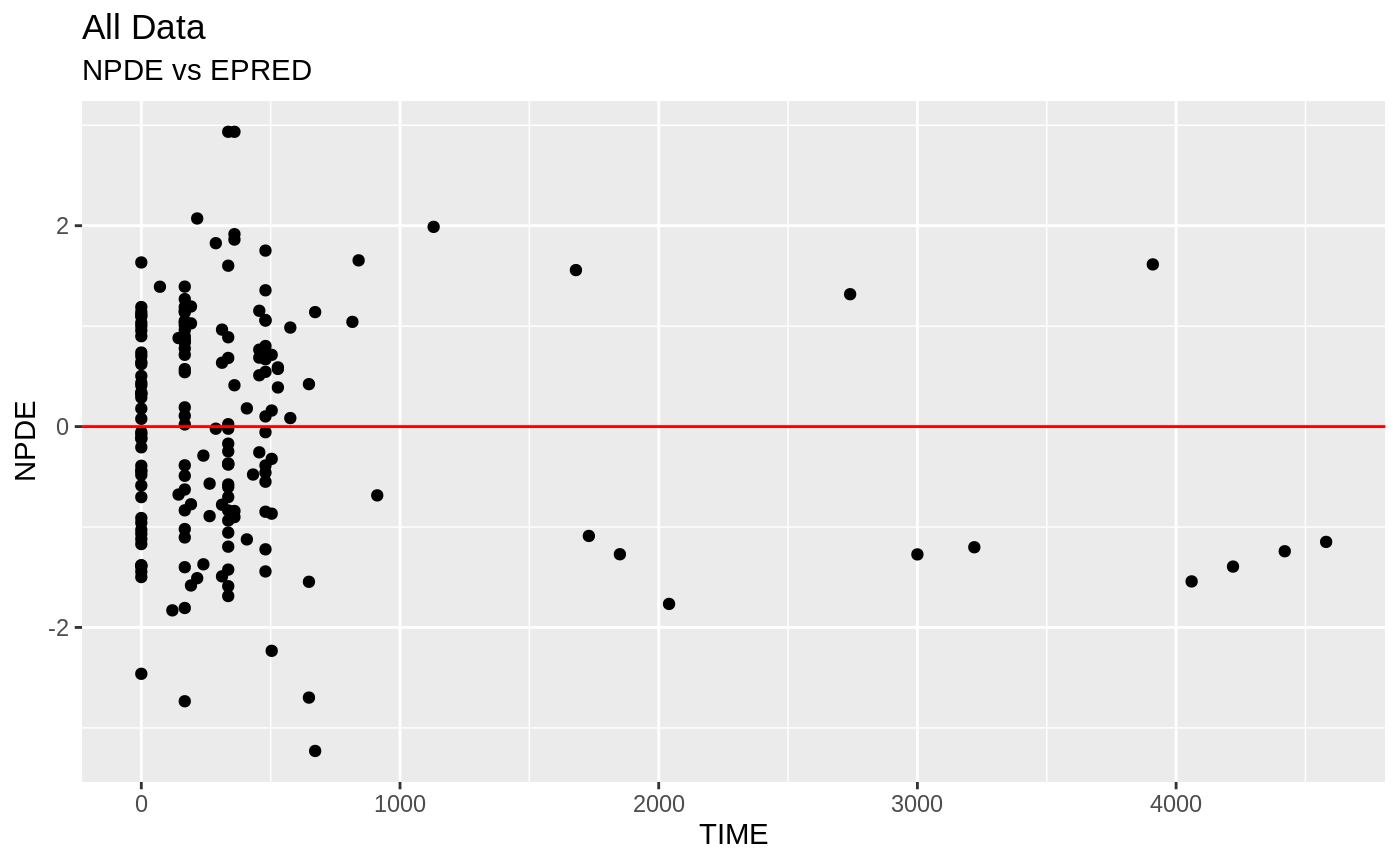
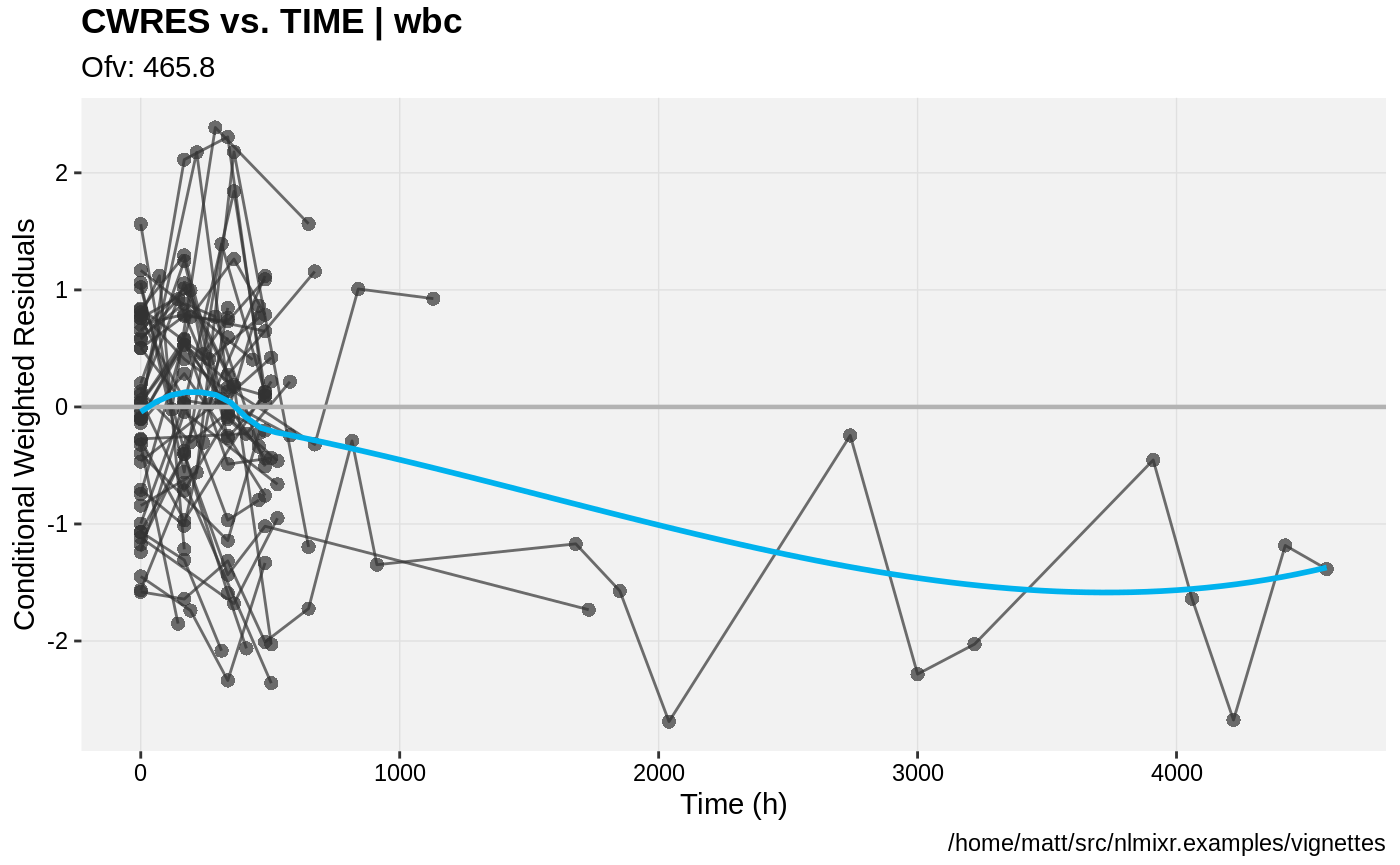
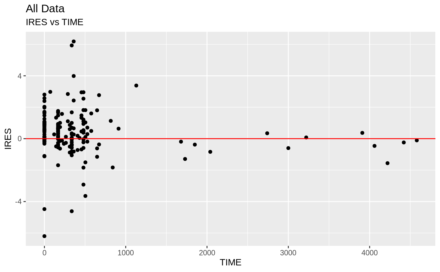
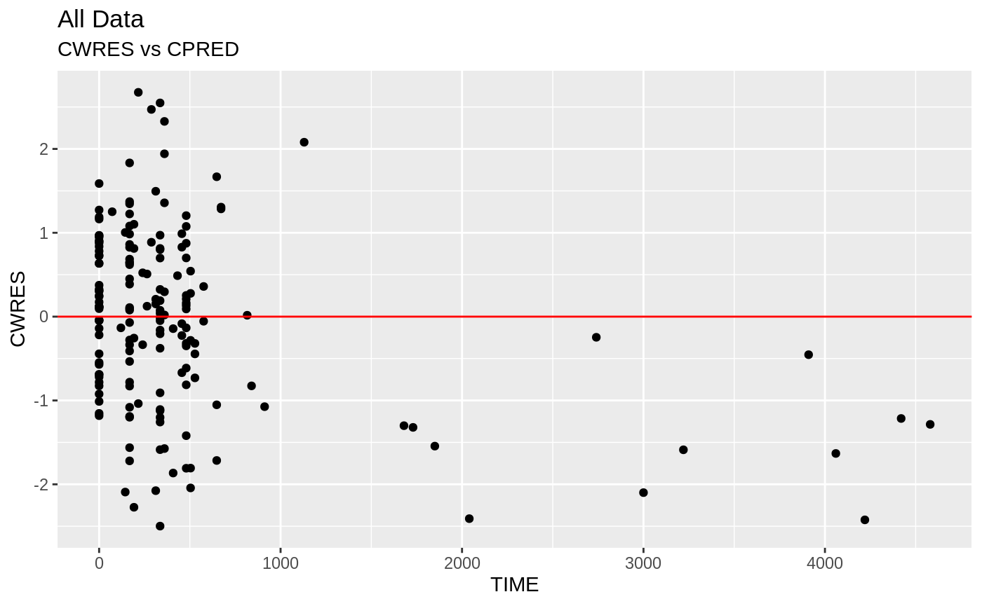
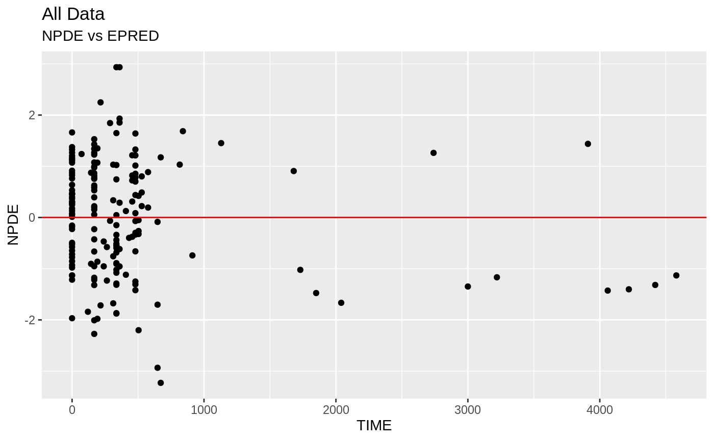
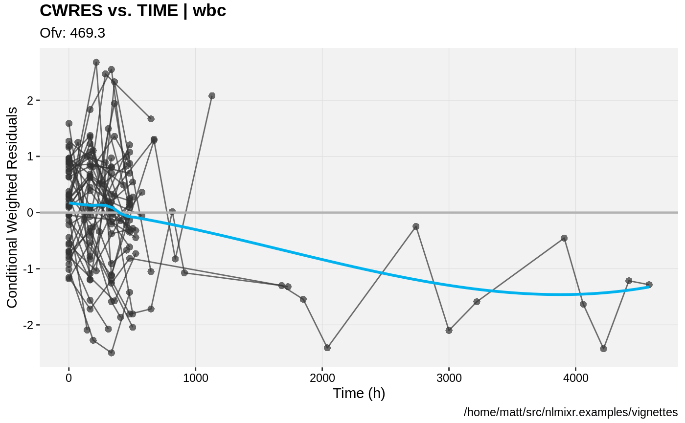
print(res_vs_idv(xpdb) +
      ylab("Conditional Weighted Residuals") +
      xlab("Time (h)"))


print(prm_vs_iteration(xpdb))


print(absval_res_vs_idv(xpdb, res = 'IWRES') +
      ylab("Individual Weighted Residuals") +
      xlab("Time (h)"))


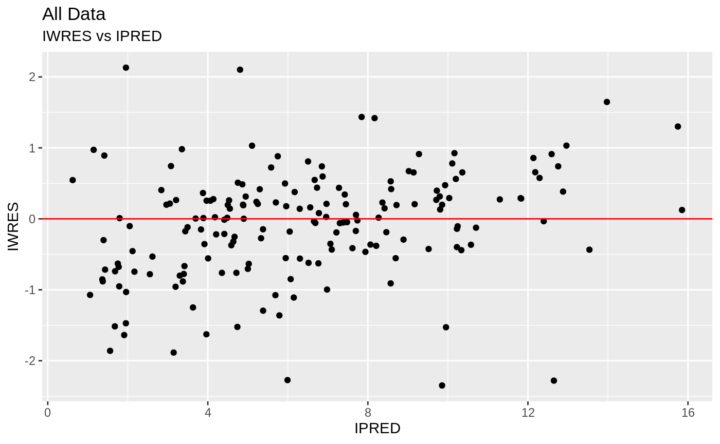
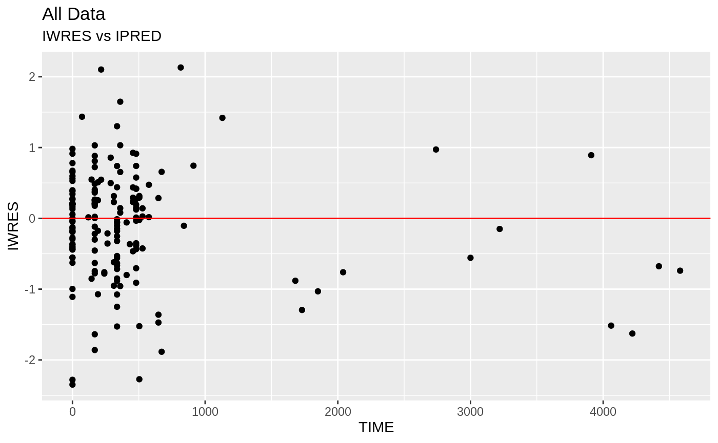
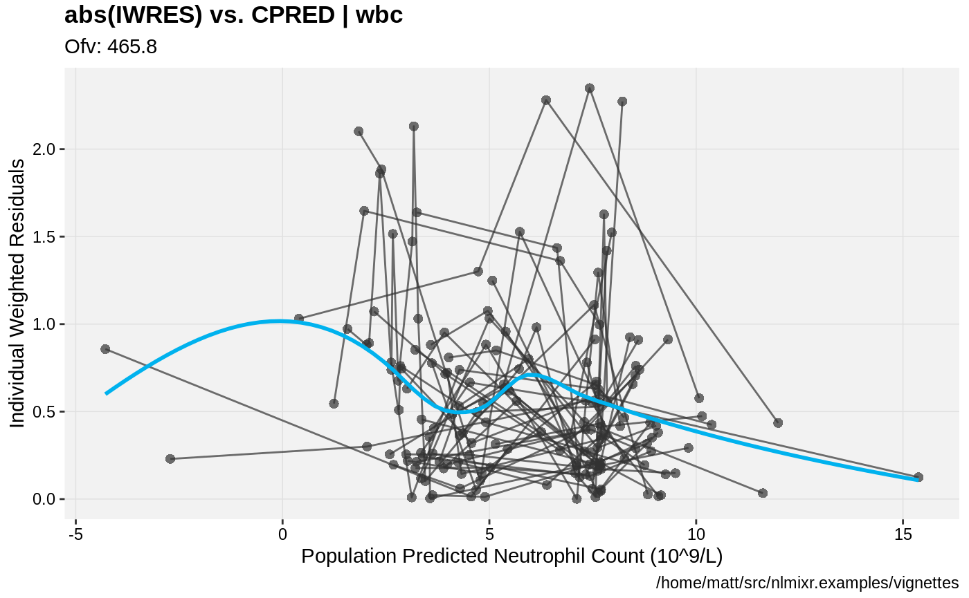
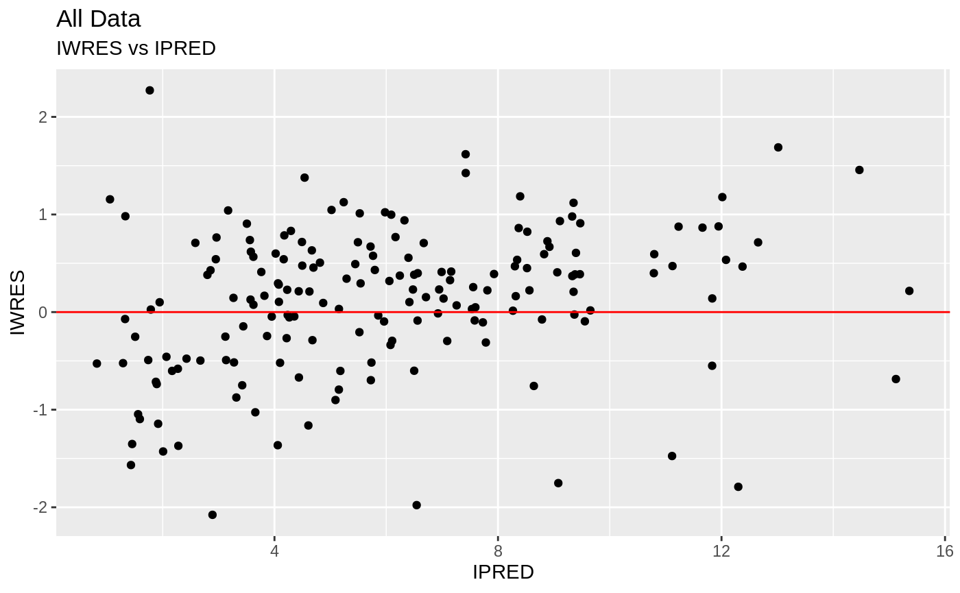
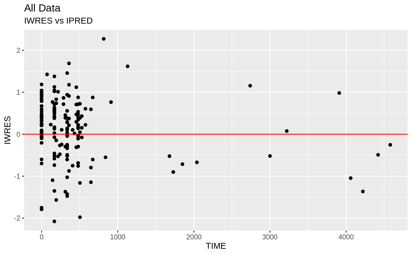
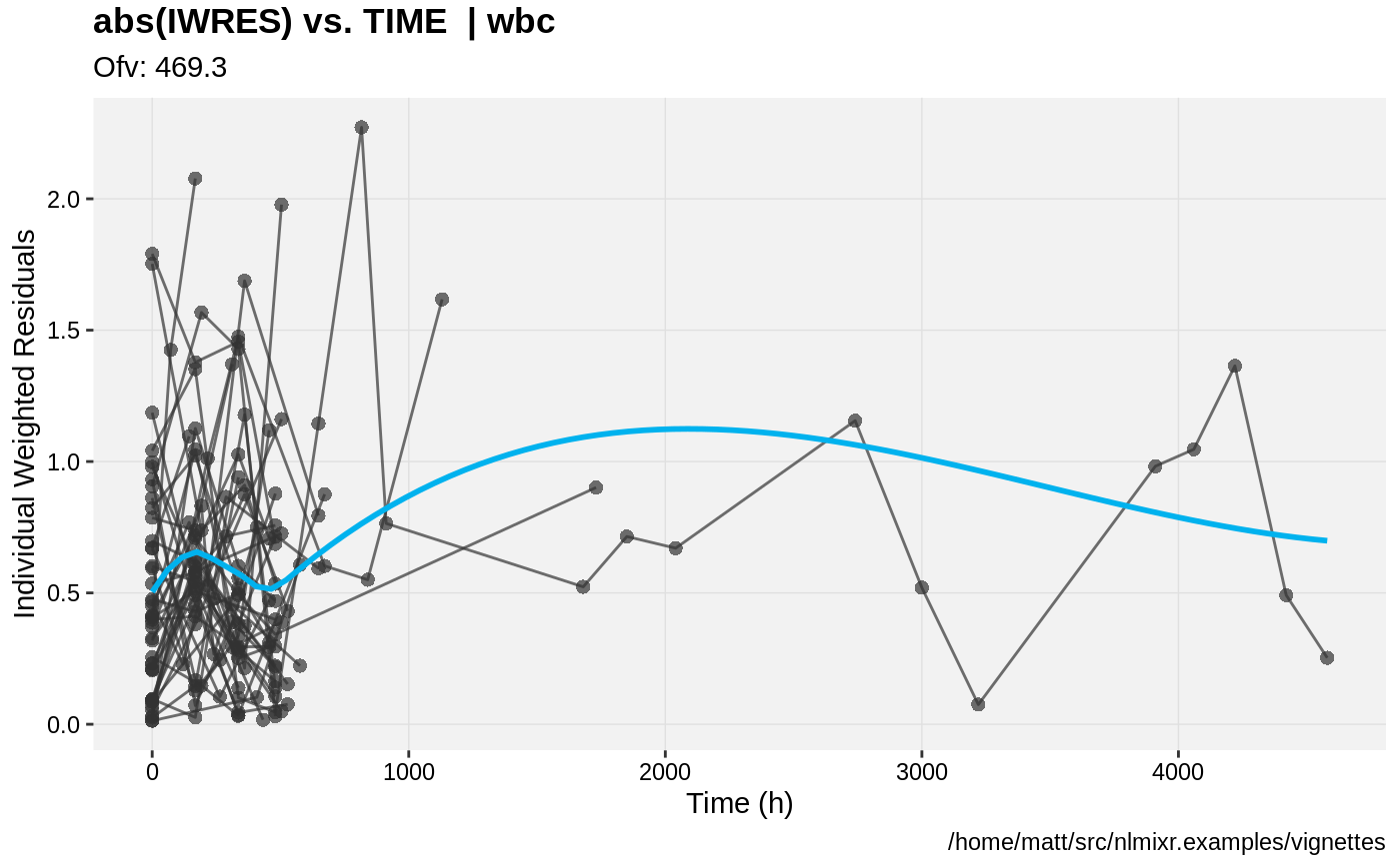
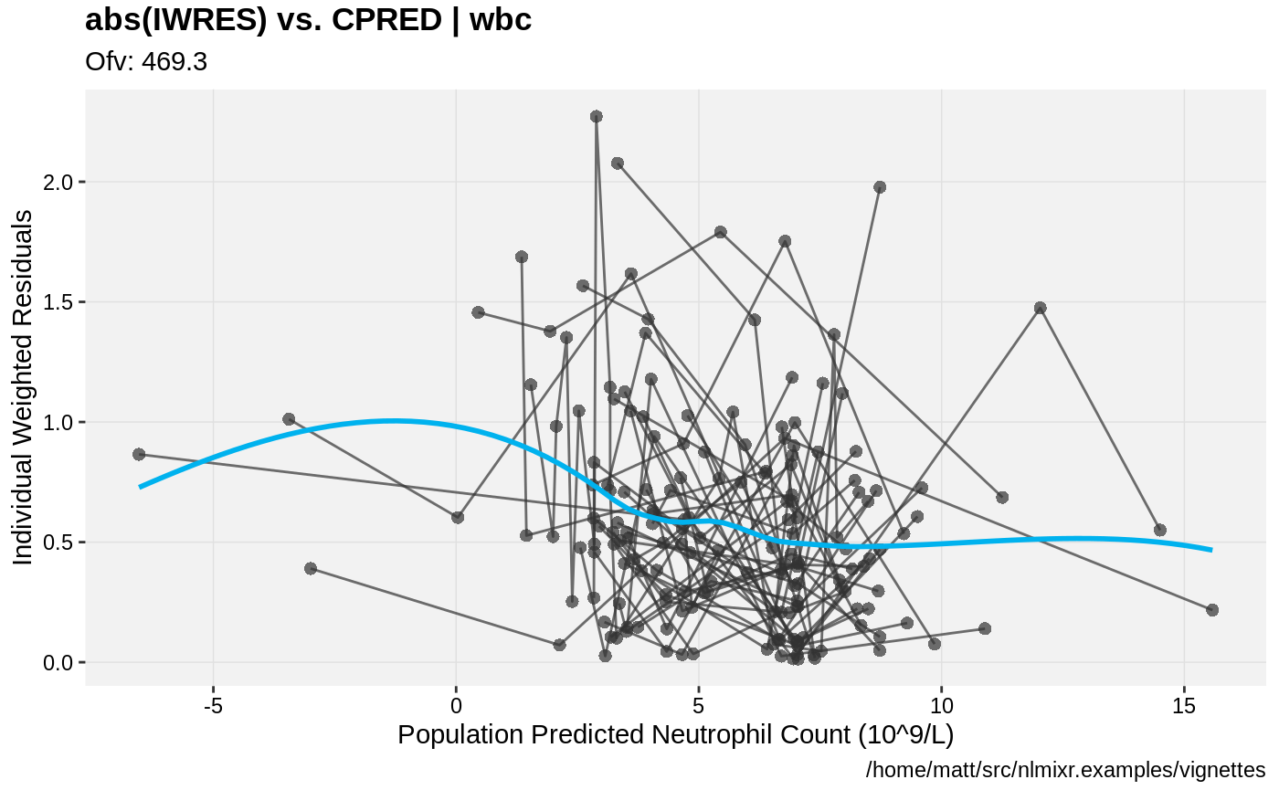
print(absval_res_vs_pred(xpdb, res = 'IWRES') +
      ylab("Individual Weighted Residuals") +
      xlab("Population Predicted Neutrophil Count (10^9/L)"))


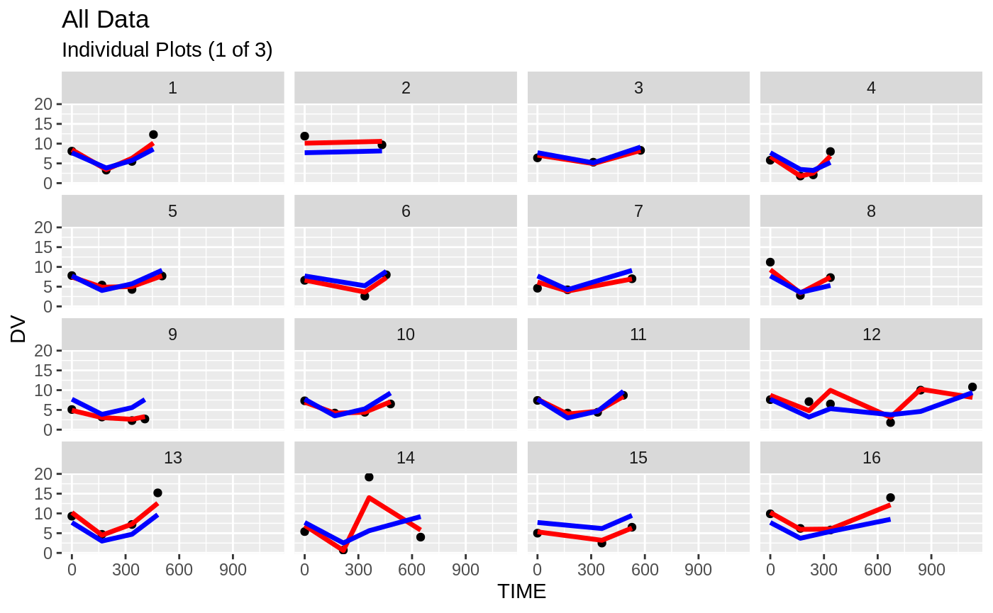
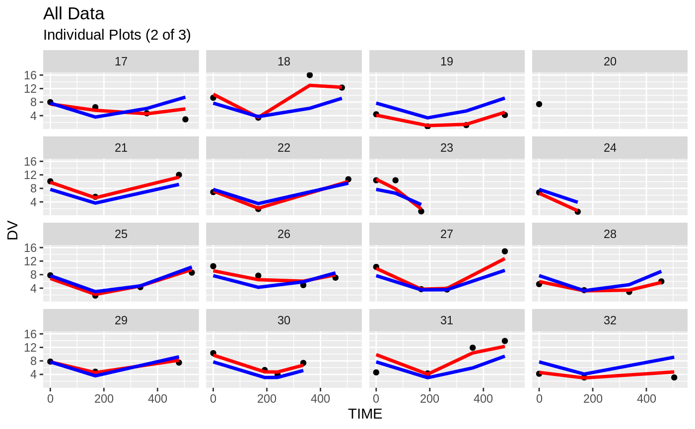
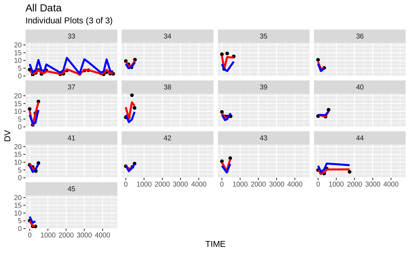
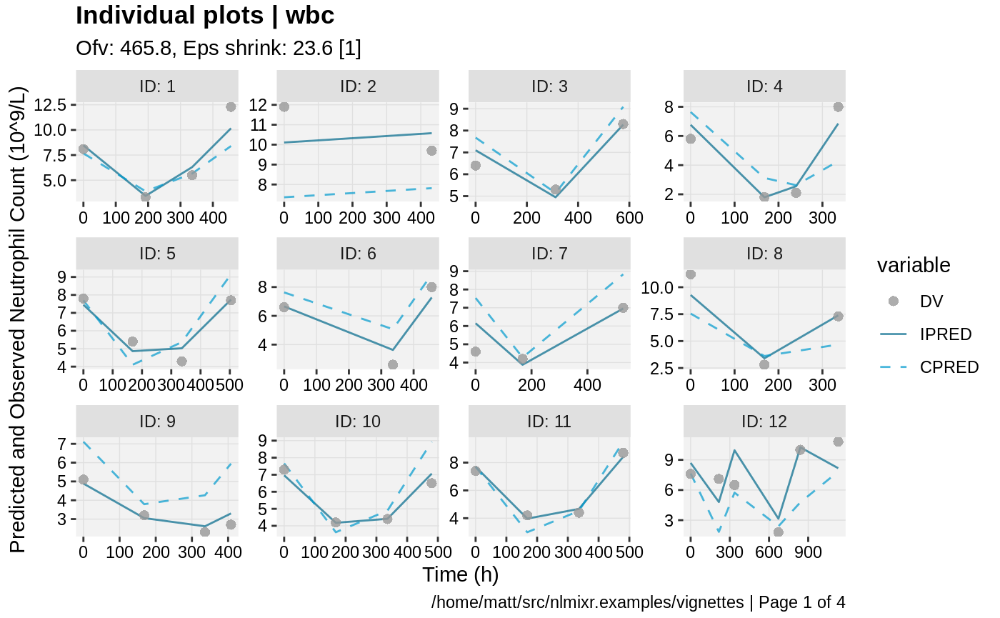
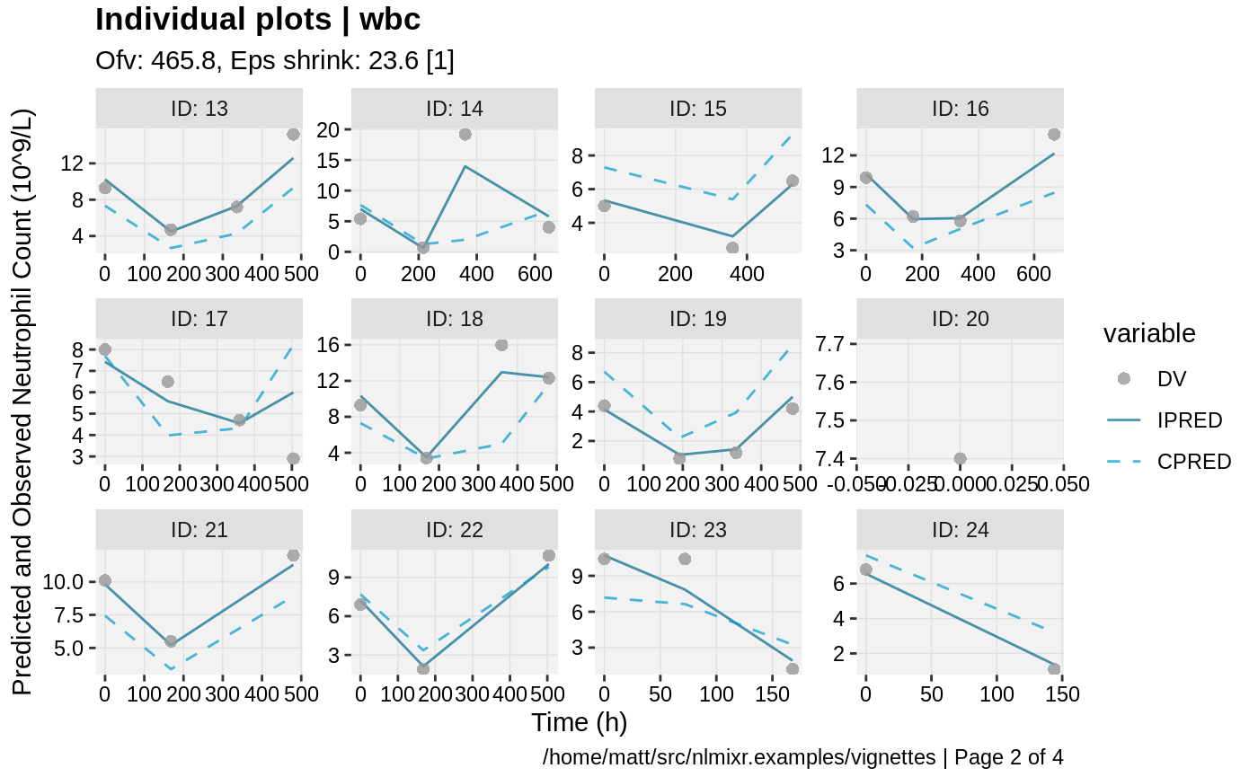
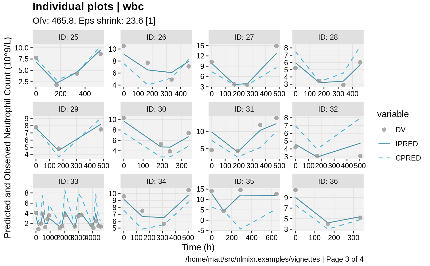
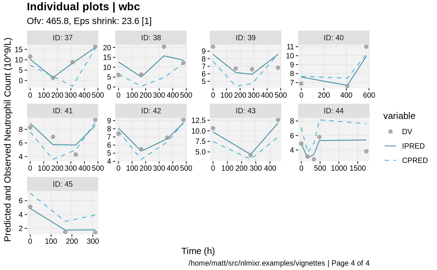
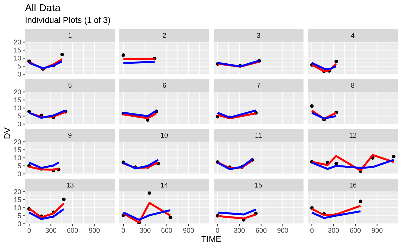
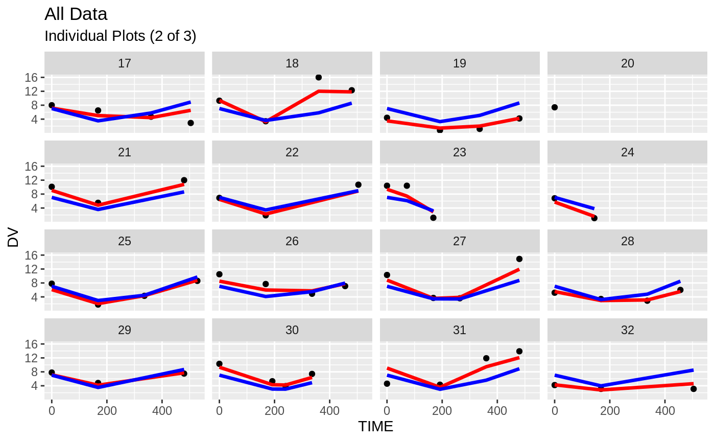
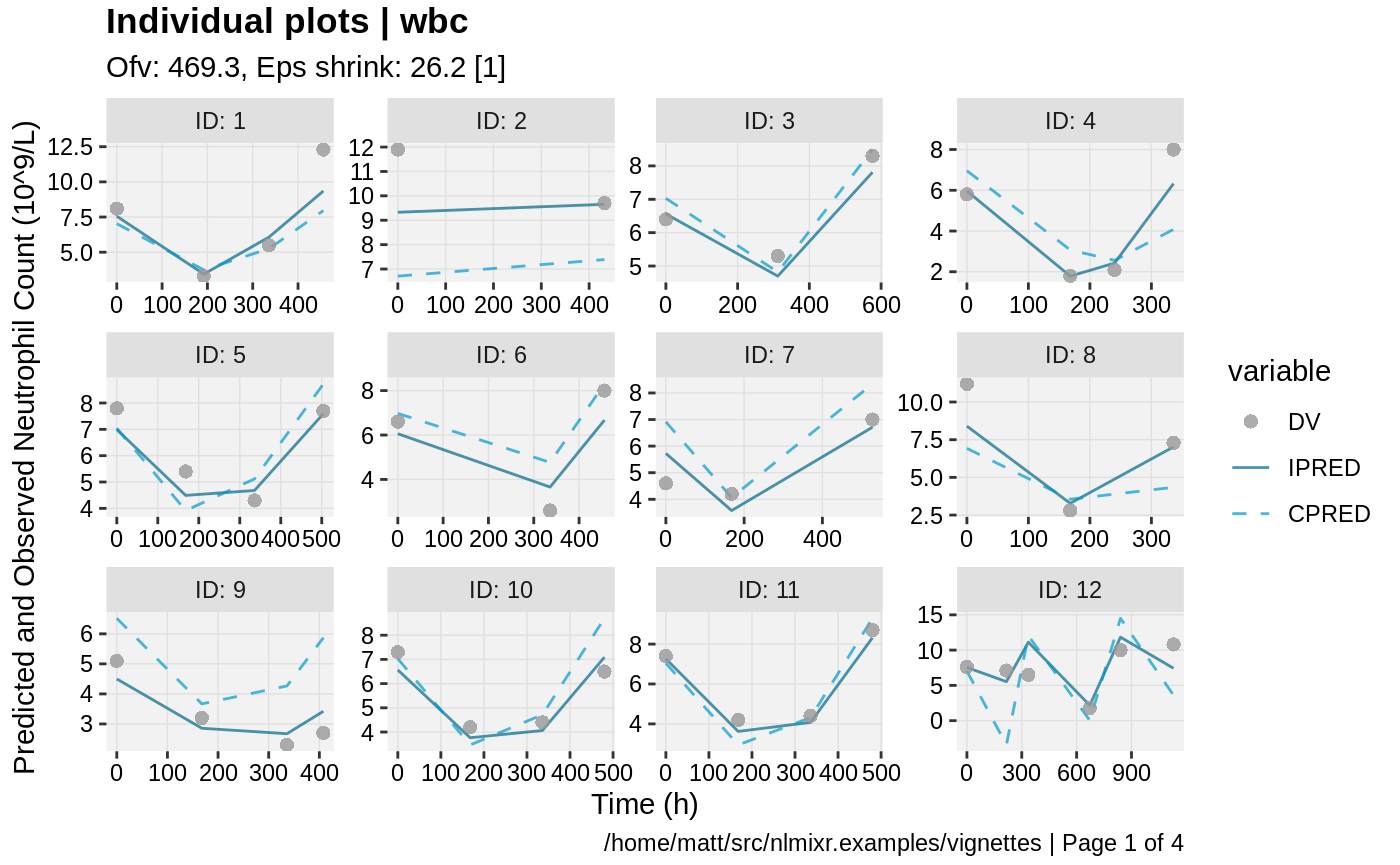
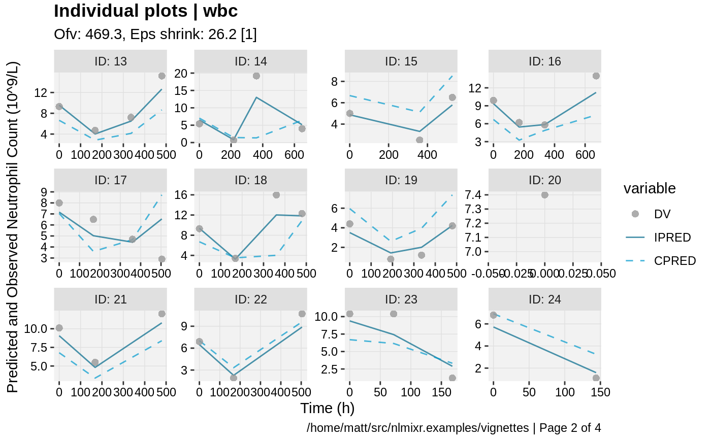
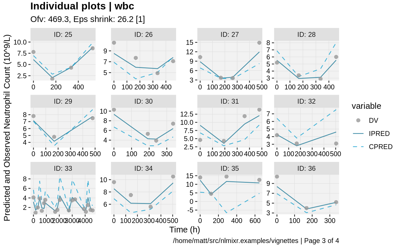
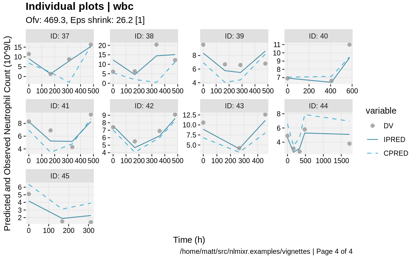
print(ind_plots(xpdb, nrow=3, ncol=4) +
      ylab("Predicted and Observed Neutrophil Count (10^9/L)") +
      xlab("Time (h)"))
#> geom_path: Each group consists of only one observation. Do you need to
#> adjust the group aesthetic?

#> geom_path: Each group consists of only one observation. Do you need to
#> adjust the group aesthetic?

#> geom_path: Each group consists of only one observation. Do you need to
#> adjust the group aesthetic?

#> geom_path: Each group consists of only one observation. Do you need to
#> adjust the group aesthetic?


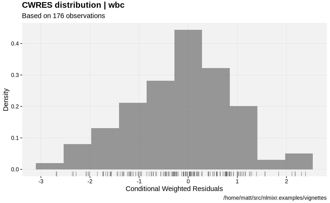
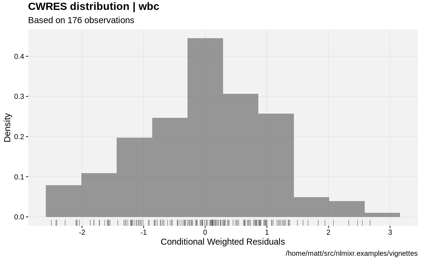
print(res_distrib(xpdb) +
      ylab("Density") +
      xlab("Conditional Weighted Residuals"))


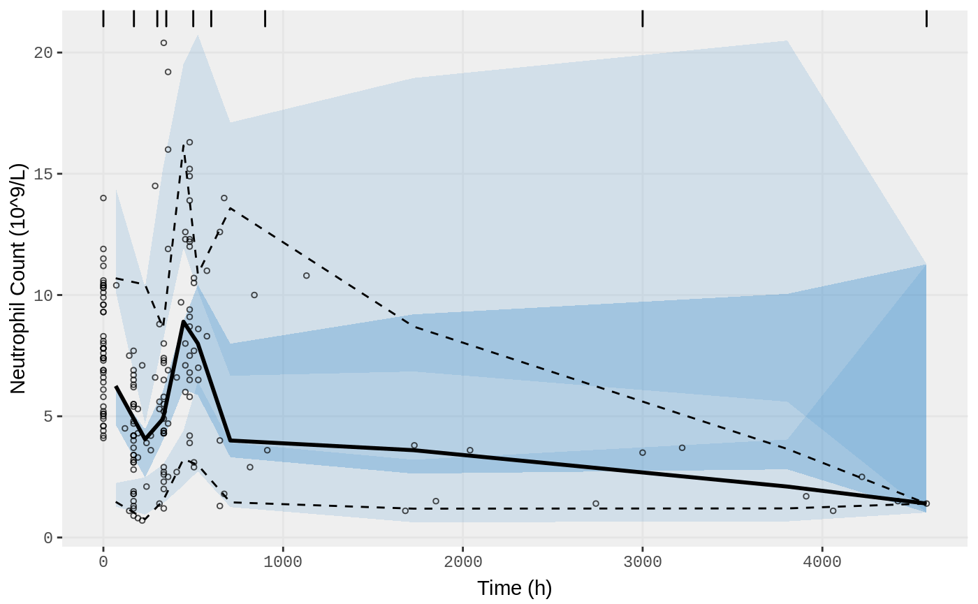
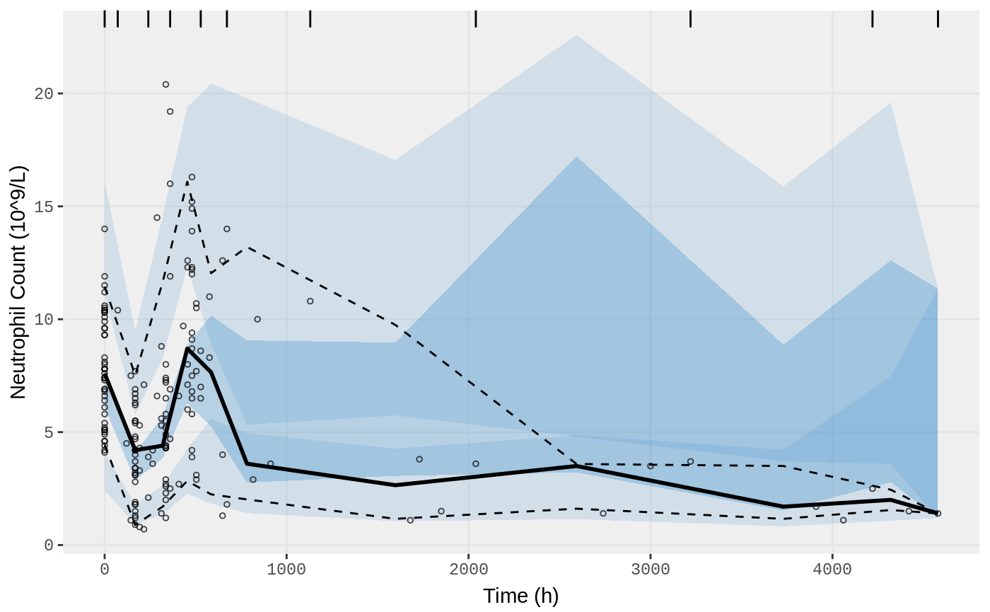
vpc.ui(fit.S, n=500, n_bins = 10, show=list(obs_dv=T), ylab = "Neutrophil Count (10^9/L)", xlab = "Time (h)")
#> Loading vpc already run (/tmp/RtmpXKdUFj/temp_libpath58be457a881a/nlmixr.examples/nlmixr-vpc-wbc-d3--57f2e50dfcdda88e020992f35b58b5f5.rds)
#>   $rxsim = original simulated data
#>   $sim = merge simulated data
#>   $obs = observed data
#>   $gg = vpc ggplot
#> use vpc(...) to change plot options
#> plotting the object now


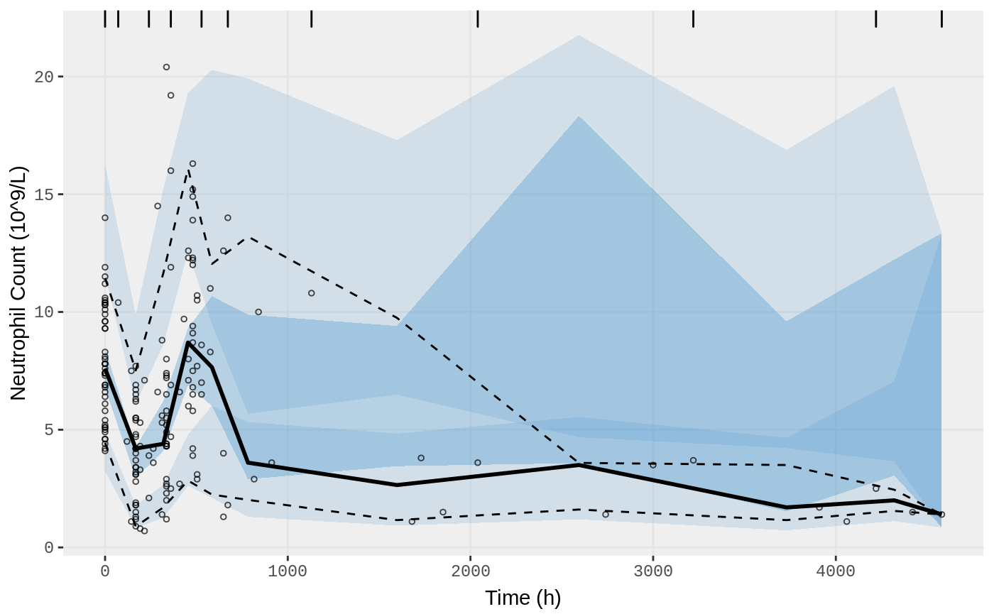
vpc.ui(fit.S, n=500, bins = c(0,170,300,350,500,600,900,3000,4580), show=list(obs_dv=T), ylab = "Neutrophil Count (10^9/L)", xlab = "Time (h)")
#> Loading vpc already run (/tmp/RtmpXKdUFj/temp_libpath58be457a881a/nlmixr.examples/nlmixr-vpc-wbc-d3--cabedf9123bd16bc37f8f5f419231637.rds)
#>   $rxsim = original simulated data
#>   $sim = merge simulated data
#>   $obs = observed data
#>   $gg = vpc ggplot
#> use vpc(...) to change plot options
#> plotting the object now

Fit model using FOCEi

fit.F <- nlmixr(wbc, d3, est="focei", table=list(cwres=TRUE, npde=TRUE))
#> Loading model already run (/tmp/RtmpXKdUFj/temp_libpath58be457a881a/nlmixr.examples/nlmixr-wbc-d3-focei-36419c3f3c6bcd0192bae24b06db4138.rds)
#> Warning in lapply(X = X, FUN = FUN, ...): ID missing in parameters dataset;
#>  Parameters are assumed to have the same order as the IDs in the event dataset
#> Warning in lapply(X = X, FUN = FUN, ...): Initial ETAs were nudged; (Can
#> control by foceiControl(etaNudge=.))
#> Warning in lapply(X = X, FUN = FUN, ...): ETAs were reset to zero during
#> optimization; (Can control by foceiControl(resetEtaP=.))
#> Warning in lapply(X = X, FUN = FUN, ...): Gradient problems with initial
#> estimate and covariance; see $scaleInfo
#> Warning in lapply(X = X, FUN = FUN, ...): Tolerances (atol/rtol) were reduced (after 5 bad solves) for some difficult ODE solving during the optimization.
#> Can control with foceiControl(stickyRecalcN=)
#> Consider reducing sigdig/atol/rtol changing initial estimates or changing the structural model.

FOCEi Goodness of fit plots

xpdb <- xpose_data_nlmixr(fit.F)
plot(fit.F)

#> geom_path: Each group consists of only one observation. Do you need to
#> adjust the group aesthetic?
#> geom_path: Each group consists of only one observation. Do you need to
#> adjust the group aesthetic?

print(dv_vs_pred(xpdb) +
      ylab("Observed Neutrophil Count (10^9/L)") +
      xlab("Population Predicted Neutrophil Count (10^9/L)"))


print(dv_vs_ipred(xpdb) +
      ylab("Observed Neutrophil Count (10^9/L)") +
      xlab("Individual Predicted Neutrophil Count (10^9/L)"))


print(res_vs_pred(xpdb) +
      ylab("Conditional Weighted Residuals") +
      xlab("Population Predicted Neutrophil Count (10^9/L)"))


print(res_vs_idv(xpdb) +
      ylab("Conditional Weighted Residuals") +
      xlab("Time (h)"))


print(absval_res_vs_idv(xpdb, res = 'IWRES') +
      ylab("Individual Weighted Residuals") +
      xlab("Time (h)"))


print(absval_res_vs_pred(xpdb, res = 'IWRES') +
      ylab("Individual Weighted Residuals") +
      xlab("Population Predicted Neutrophil Count (10^9/L)"))


print(ind_plots(xpdb, nrow=3, ncol=4) +
      ylab("Predicted and Observed Neutrophil Count (10^9/L)") +
      xlab("Time (h)"))
#> geom_path: Each group consists of only one observation. Do you need to
#> adjust the group aesthetic?

#> geom_path: Each group consists of only one observation. Do you need to
#> adjust the group aesthetic?

#> geom_path: Each group consists of only one observation. Do you need to
#> adjust the group aesthetic?

#> geom_path: Each group consists of only one observation. Do you need to
#> adjust the group aesthetic?


print(res_distrib(xpdb) +
      ylab("Density") +
      xlab("Conditional Weighted Residuals"))


#vpc.ui(fit.S, n=500, show=list(obs_dv=T), ylab = "Neutrophil count (10^9/L)", xlab = "Time (h)")
# 10 bins is slightly better than auto bin
vpc.ui(fit.F, n=500, n_bins = 10, show=list(obs_dv=T), ylab = "Neutrophil Count (10^9/L)", xlab = "Time (h)")
#> Loading vpc already run (/tmp/RtmpXKdUFj/temp_libpath58be457a881a/nlmixr.examples/nlmixr-vpc-wbc-d3--c2e7b79f91651851066ecd8d902c91ee.rds)
#>   $rxsim = original simulated data
#>   $sim = merge simulated data
#>   $obs = observed data
#>   $gg = vpc ggplot
#> use vpc(...) to change plot options
#> plotting the object now


# specify bins
vpc.ui(fit.F, n=500, bins = c(0,170,300,350,500,600,900,3000,4580), show=list(obs_dv=T), ylab = "Neutrophil Count (10^9/L)", xlab = "Time (h)")
#> Loading vpc already run (/tmp/RtmpXKdUFj/temp_libpath58be457a881a/nlmixr.examples/nlmixr-vpc-wbc-d3--bb99abc56c26bc0e6220829df60cd738.rds)
#>   $rxsim = original simulated data
#>   $sim = merge simulated data
#>   $obs = observed data
#>   $gg = vpc ggplot
#> use vpc(...) to change plot options
#> plotting the object now

Friberg Myelosuppression model

Yuan Xiong

Fit model using saem

Fit model using FOCEi

FOCEi Goodness of fit plots

Contents