mavoglurant – Physiologically-based PK

Wenping Wang

2019-10-17

nlmixr

Building on the first simple example, we can be more ambitious, and try a full PBPK model. This one was published for mavoglurant (Wendling et al. 2016).

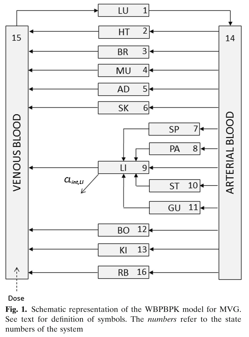
Model Schematic

nlmixr model

library(nlmixr)

library(xpose)
#> Loading required package: ggplot2
#> 
#> Attaching package: 'xpose'
#> The following object is masked from 'package:nlmixr':
#> 
#>     vpc
#> The following object is masked from 'package:stats':
#> 
#>     filter
library(xpose.nlmixr)
#> 
#> Attaching package: 'xpose.nlmixr'
#> The following object is masked from 'package:nlmixr':
#> 
#>     vpc
library(ggplot2)

pbpk <- function(){
    ini({
        ##theta=exp(c(1.1, .3, 2, 7.6, .003, .3))
        lKbBR = 1.1
        lKbMU = 0.3
        lKbAD = 2
        lCLint = 7.6
        lKbBO = 0.03
        lKbRB = 0.3
        eta.LClint ~ 4
        add.err <- 1
        prop.err <- 10
    })
    model({
        KbBR = exp(lKbBR)
        KbMU = exp(lKbMU)
        KbAD = exp(lKbAD)
        CLint= exp(lCLint + eta.LClint)
        KbBO = exp(lKbBO)
        KbRB = exp(lKbRB)

        ## Regional blood flows
        CO  = (187.00*WT^0.81)*60/1000;         # Cardiac output (L/h) from White et al (1968)
        QHT = 4.0 *CO/100;
        QBR = 12.0*CO/100;
        QMU = 17.0*CO/100;
        QAD = 5.0 *CO/100;
        QSK = 5.0 *CO/100;
        QSP = 3.0 *CO/100;
        QPA = 1.0 *CO/100;
        QLI = 25.5*CO/100;
        QST = 1.0 *CO/100;
        QGU = 14.0*CO/100;
        QHA = QLI - (QSP + QPA + QST + QGU); # Hepatic artery blood flow
        QBO = 5.0 *CO/100;
        QKI = 19.0*CO/100;
        QRB = CO - (QHT + QBR + QMU + QAD + QSK + QLI + QBO + QKI);
        QLU = QHT + QBR + QMU + QAD + QSK + QLI + QBO + QKI + QRB;

        ## Organs' volumes = organs' weights / organs' density
        VLU = (0.76 *WT/100)/1.051;
        VHT = (0.47 *WT/100)/1.030;
        VBR = (2.00 *WT/100)/1.036;
        VMU = (40.00*WT/100)/1.041;
        VAD = (21.42*WT/100)/0.916;
        VSK = (3.71 *WT/100)/1.116;
        VSP = (0.26 *WT/100)/1.054;
        VPA = (0.14 *WT/100)/1.045;
        VLI = (2.57 *WT/100)/1.040;
        VST = (0.21 *WT/100)/1.050;
        VGU = (1.44 *WT/100)/1.043;
        VBO = (14.29*WT/100)/1.990;
        VKI = (0.44 *WT/100)/1.050;
        VAB = (2.81 *WT/100)/1.040;
        VVB = (5.62 *WT/100)/1.040;
        VRB = (3.86 *WT/100)/1.040;

        ## Fixed parameters
        BP = 0.61;      # Blood:plasma partition coefficient
        fup = 0.028;    # Fraction unbound in plasma
        fub = fup/BP;   # Fraction unbound in blood

        KbLU = exp(0.8334);
        KbHT = exp(1.1205);
        KbSK = exp(-.5238);
        KbSP = exp(0.3224);
        KbPA = exp(0.3224);
        KbLI = exp(1.7604);
        KbST = exp(0.3224);
        KbGU = exp(1.2026);
        KbKI = exp(1.3171);

        ##-----------------------------------------
        S15 = VVB*BP/1000;
        C15 = Venous_Blood/S15

        ##-----------------------------------------
        d/dt(Lungs) = QLU*(Venous_Blood/VVB - Lungs/KbLU/VLU);
        d/dt(Heart) = QHT*(Arterial_Blood/VAB - Heart/KbHT/VHT);
        d/dt(Brain) = QBR*(Arterial_Blood/VAB - Brain/KbBR/VBR);
        d/dt(Muscles) = QMU*(Arterial_Blood/VAB - Muscles/KbMU/VMU);
        d/dt(Adipose) = QAD*(Arterial_Blood/VAB - Adipose/KbAD/VAD);
        d/dt(Skin) = QSK*(Arterial_Blood/VAB - Skin/KbSK/VSK);
        d/dt(Spleen) = QSP*(Arterial_Blood/VAB - Spleen/KbSP/VSP);
        d/dt(Pancreas) = QPA*(Arterial_Blood/VAB - Pancreas/KbPA/VPA);
        d/dt(Liver) = QHA*Arterial_Blood/VAB + QSP*Spleen/KbSP/VSP + QPA*Pancreas/KbPA/VPA + QST*Stomach/KbST/VST + QGU*Gut/KbGU/VGU - CLint*fub*Liver/KbLI/VLI - QLI*Liver/KbLI/VLI;
        d/dt(Stomach) = QST*(Arterial_Blood/VAB - Stomach/KbST/VST);
        d/dt(Gut) = QGU*(Arterial_Blood/VAB - Gut/KbGU/VGU);
        d/dt(Bones) = QBO*(Arterial_Blood/VAB - Bones/KbBO/VBO);
        d/dt(Kidneys) = QKI*(Arterial_Blood/VAB - Kidneys/KbKI/VKI);
        d/dt(Arterial_Blood) = QLU*(Lungs/KbLU/VLU - Arterial_Blood/VAB);
        d/dt(Venous_Blood) = QHT*Heart/KbHT/VHT + QBR*Brain/KbBR/VBR + QMU*Muscles/KbMU/VMU + QAD*Adipose/KbAD/VAD + QSK*Skin/KbSK/VSK + QLI*Liver/KbLI/VLI + QBO*Bones/KbBO/VBO + QKI*Kidneys/KbKI/VKI + QRB*Rest_of_Body/KbRB/VRB - QLU*Venous_Blood/VVB;
        d/dt(Rest_of_Body) = QRB*(Arterial_Blood/VAB - Rest_of_Body/KbRB/VRB);

        C15 ~ add(add.err) + prop(prop.err)
    })
}

dat = read.csv("Mavoglurant_A2121_nmpk.csv")
dat$occ = unlist(with(dat, tapply(EVID, ID, function(x) cumsum(x>0))))
dat = subset(dat, occ==1)
dat = subset(dat, ID<812) ## First 20
dat = subset(dat, EVID>0 | DV>0)
dat$CMT[dat$CMT == 0]  <- 1;
dat$CMT[dat$EVID == 1]  <- "Venous_Blood" ## Compartment dosed to is Venous Blood
dat$CMT[dat$EVID != 1]  <- "C15" ## Observing C15

gofs <- function(fit){
    ################################################################################
    ## Standard plots
    ################################################################################
    plot(fit);

    xpdb <- xpose_data_nlmixr(fit) ## Convert to nlmixr object

    print(dv_vs_pred(xpdb) +
          ylab("Observed Mavoglurant Concentrations (ng/mL)") +
          xlab("Population Predicted Mavoglurant Concentrations (ng/mL)"));

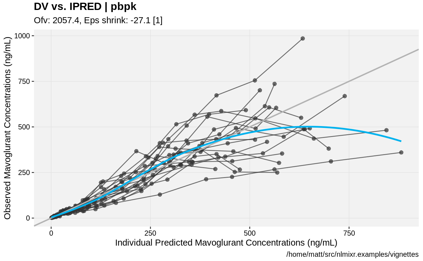
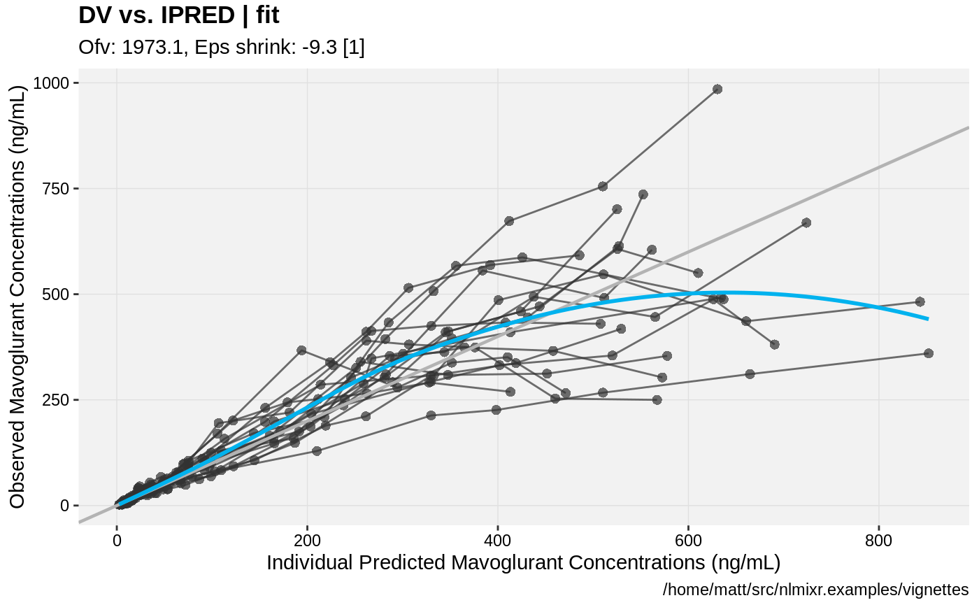
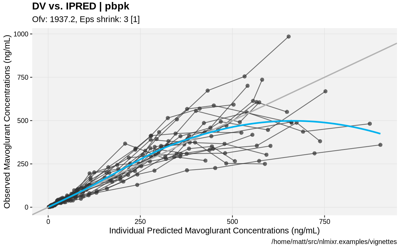
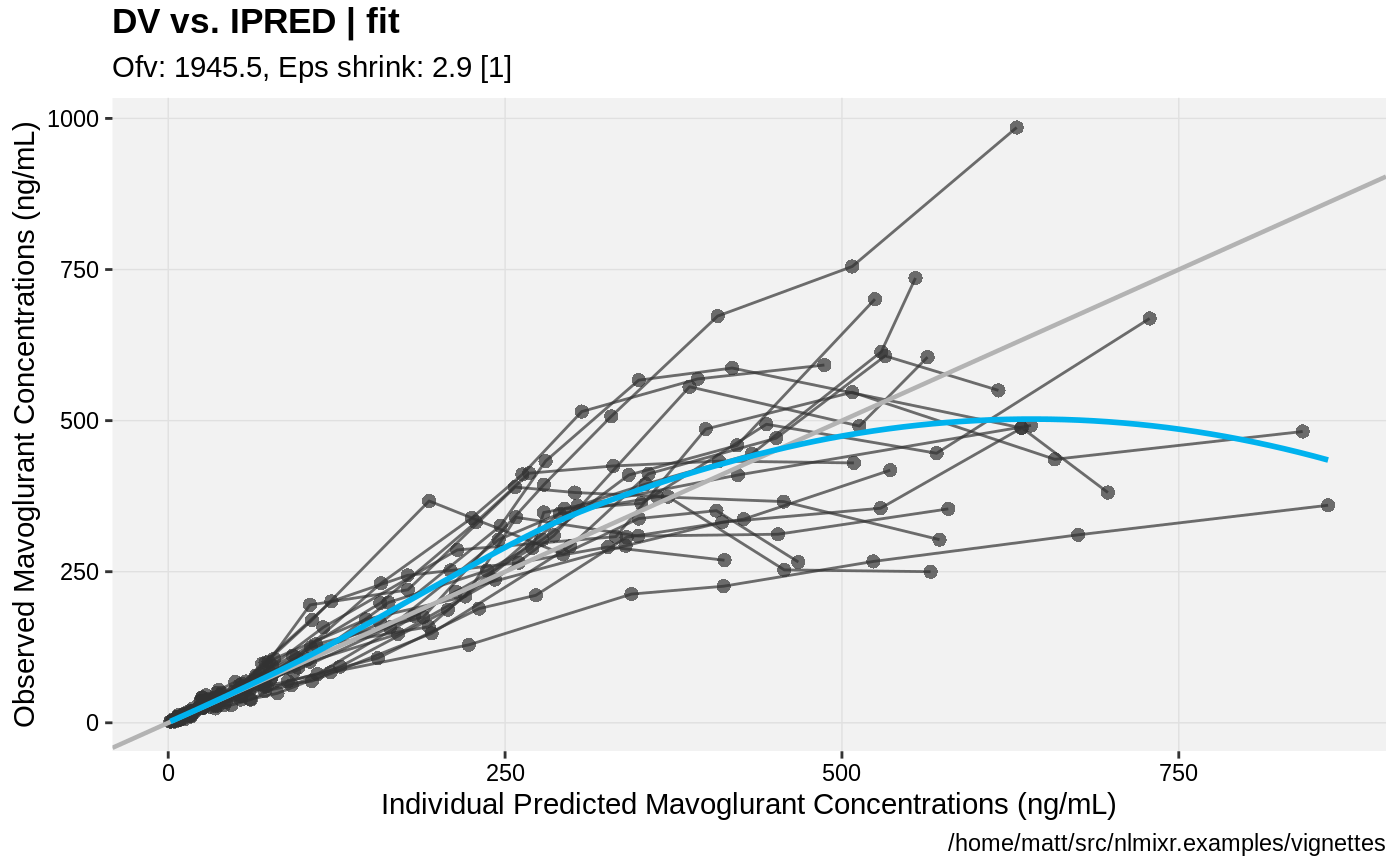
    print(dv_vs_ipred(xpdb) +
          ylab("Observed Mavoglurant Concentrations (ng/mL)") +
          xlab("Individual Predicted Mavoglurant Concentrations (ng/mL)"));

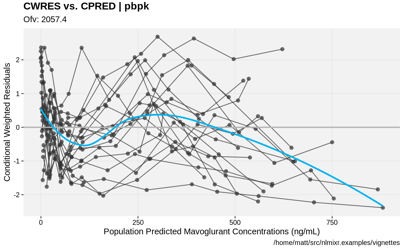
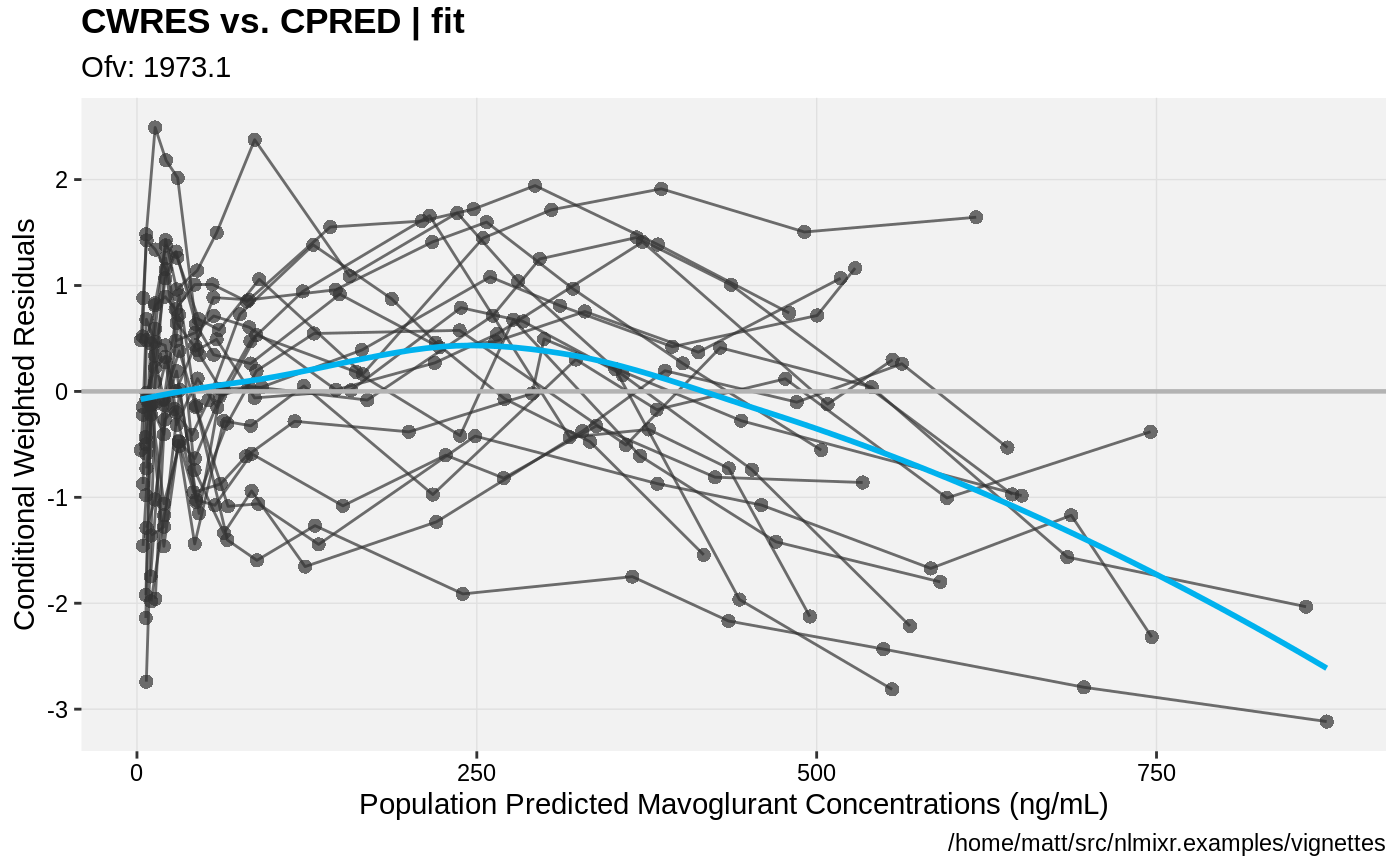
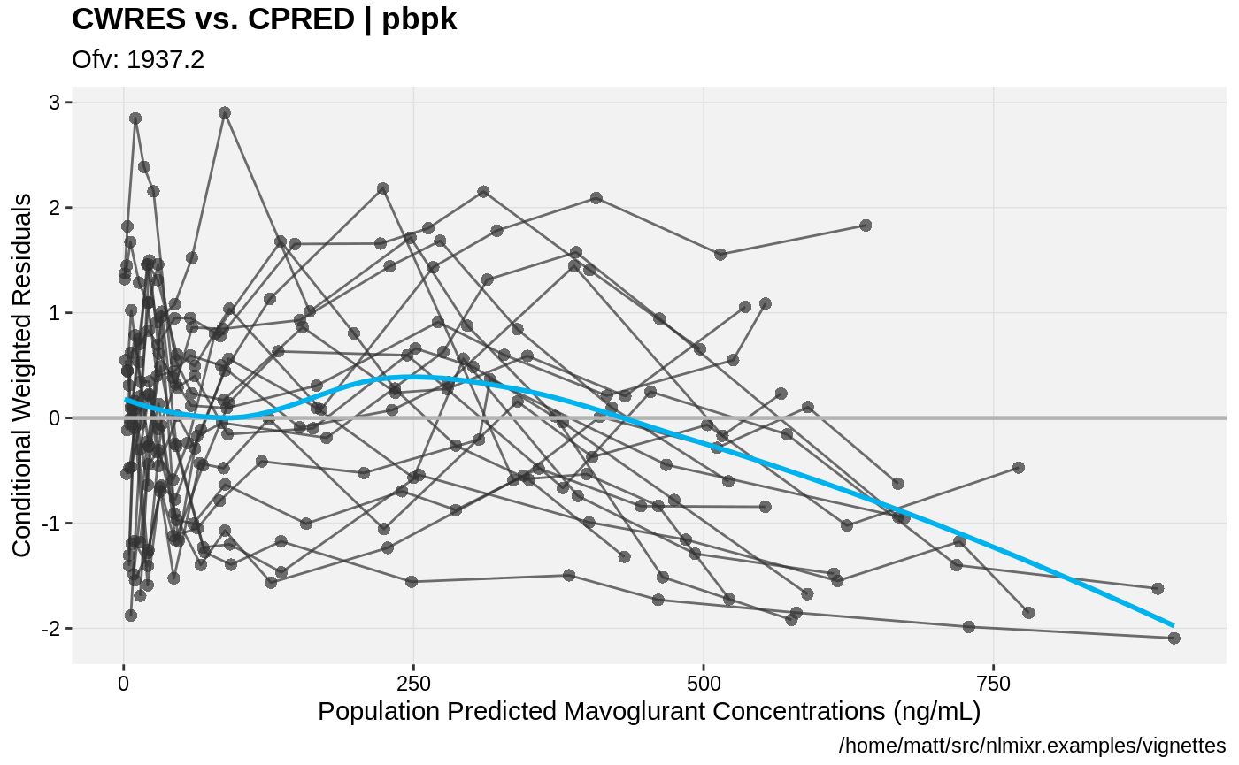
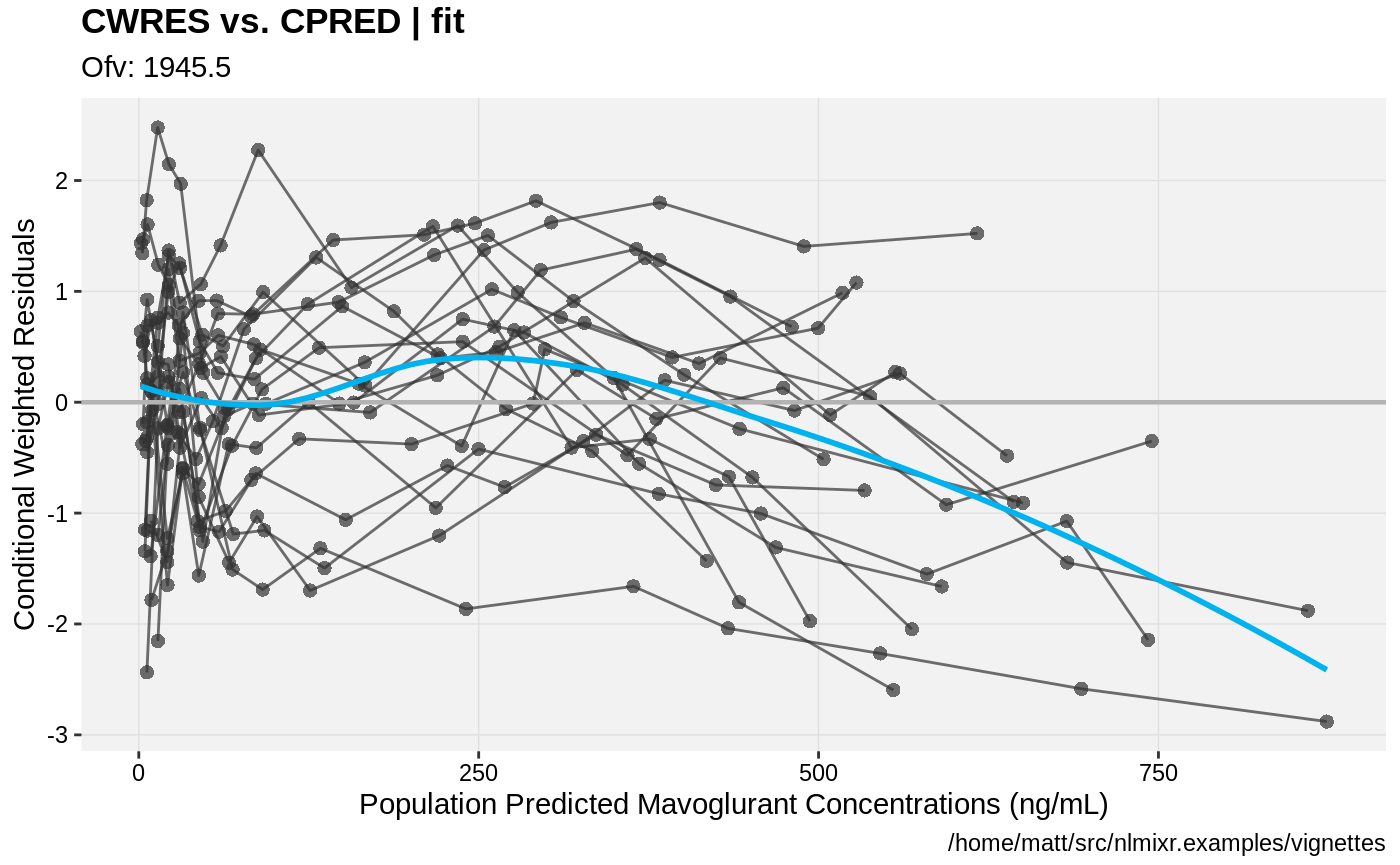
    print(res_vs_pred(xpdb) +
          ylab("Conditional Weighted Residuals") +
          xlab("Population Predicted Mavoglurant Concentrations (ng/mL)"));

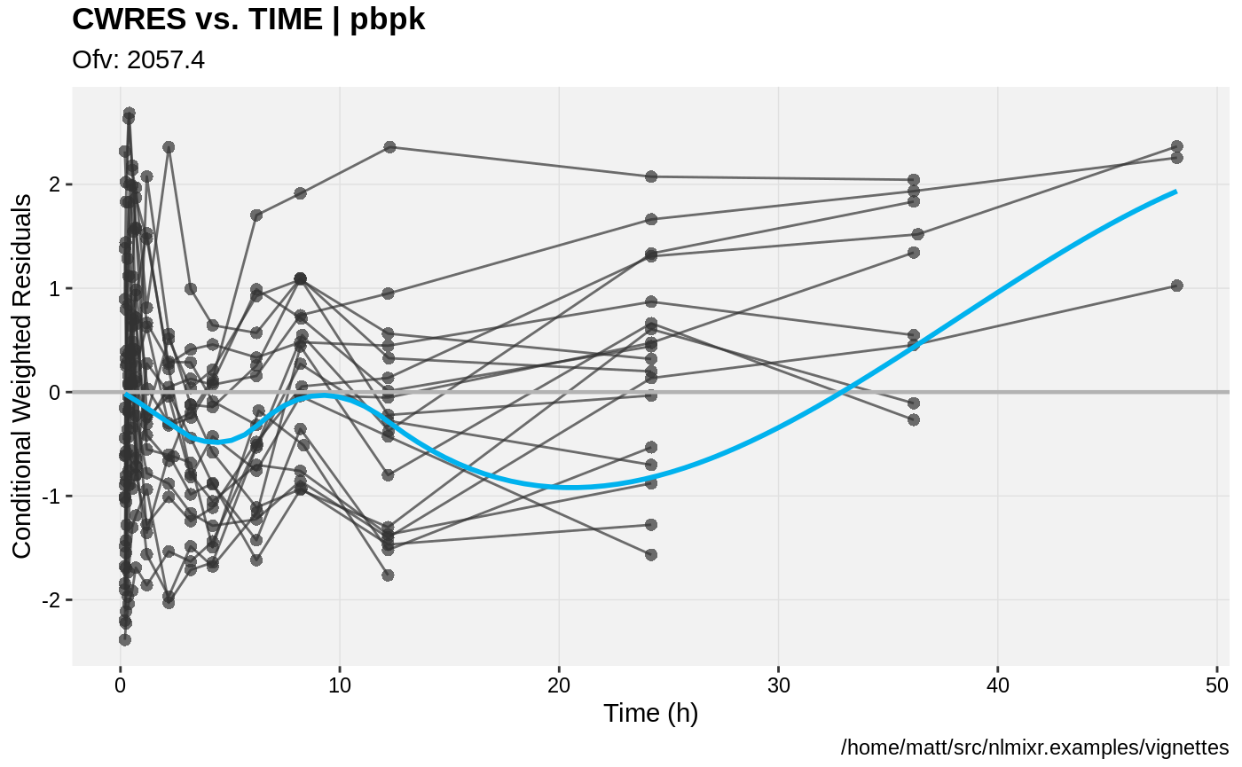
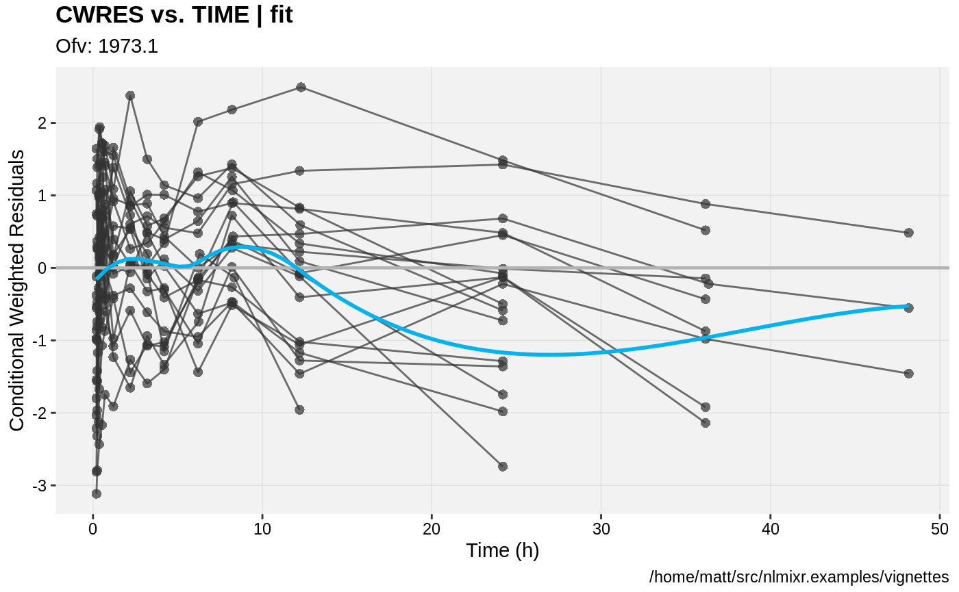
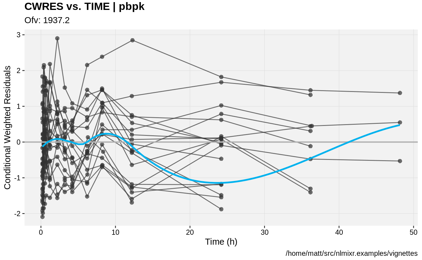
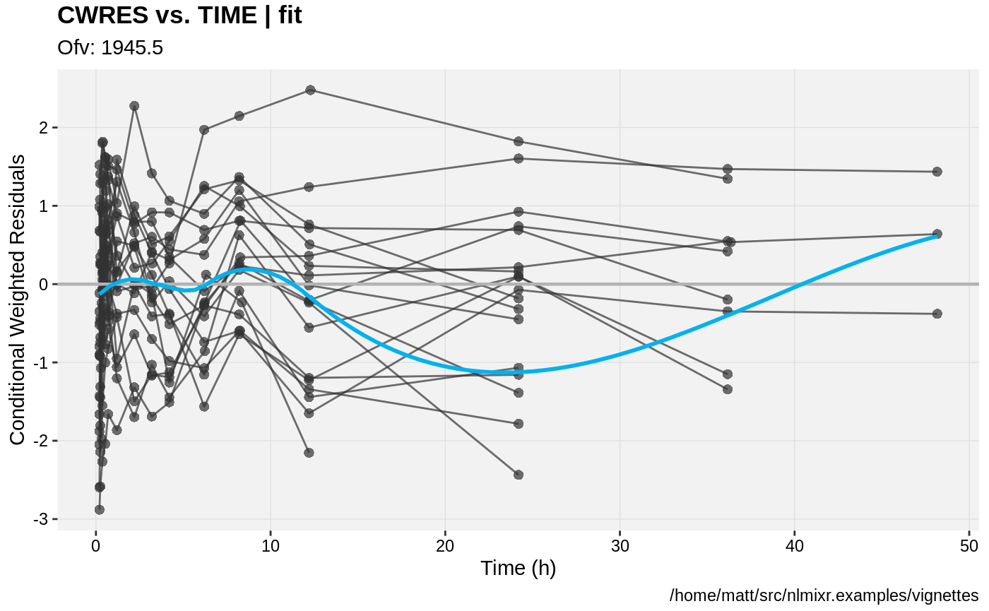
    print(res_vs_idv(xpdb) +
          ylab("Conditional Weighted Residuals") +
          xlab("Time (h)"));

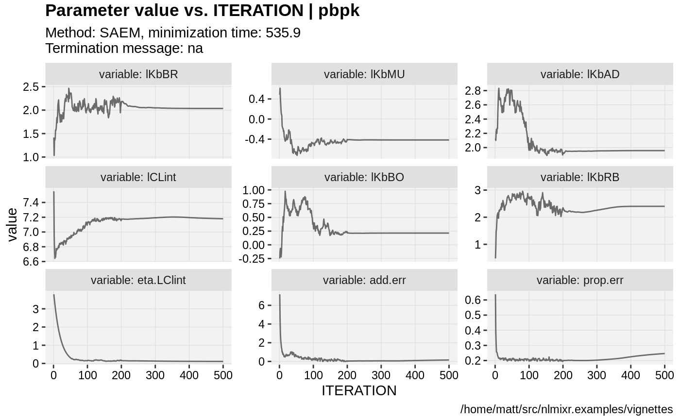
    if (!is.null(fit$saem)){
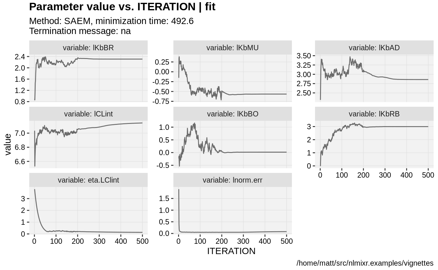
        print(prm_vs_iteration(xpdb));
    }

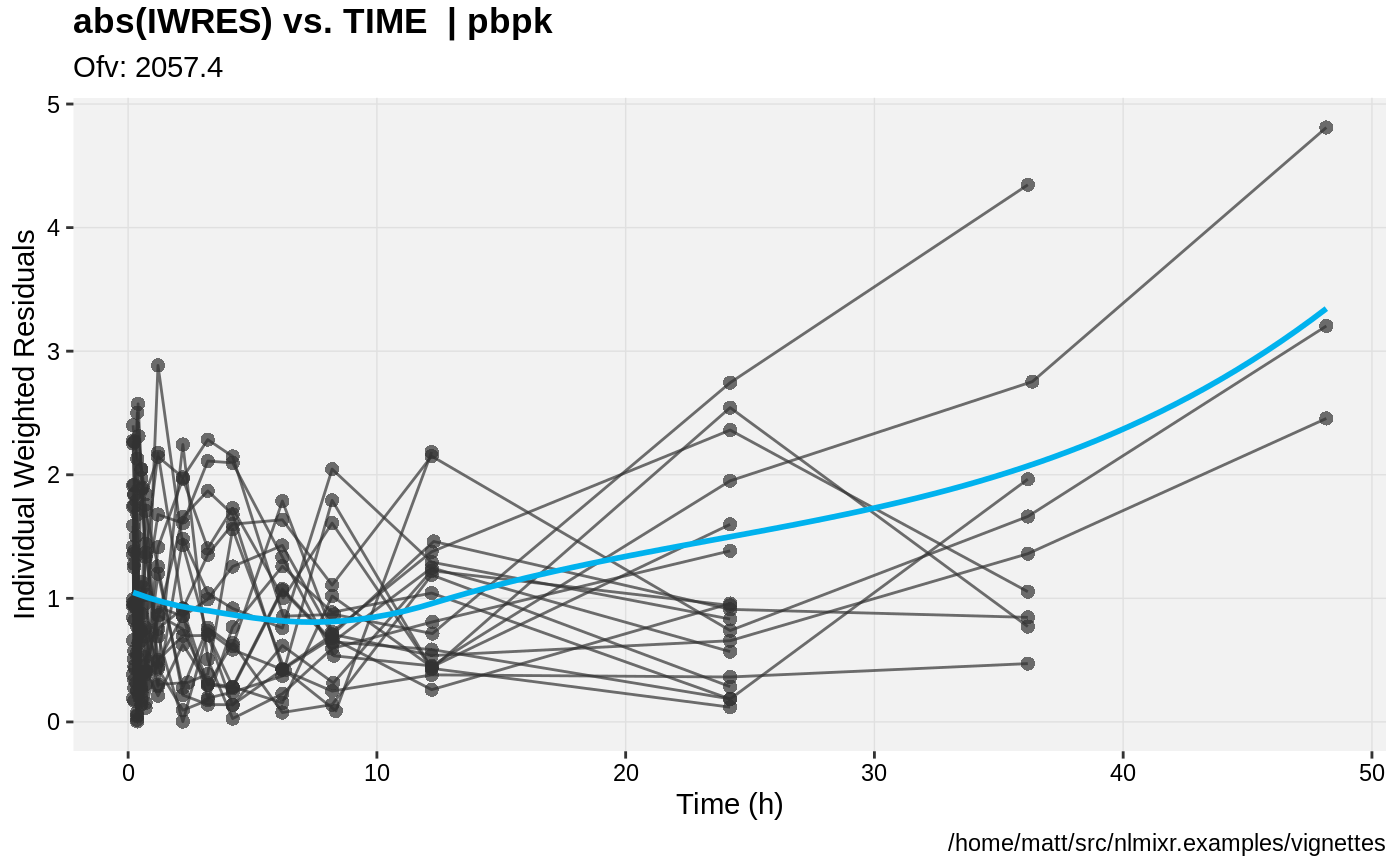
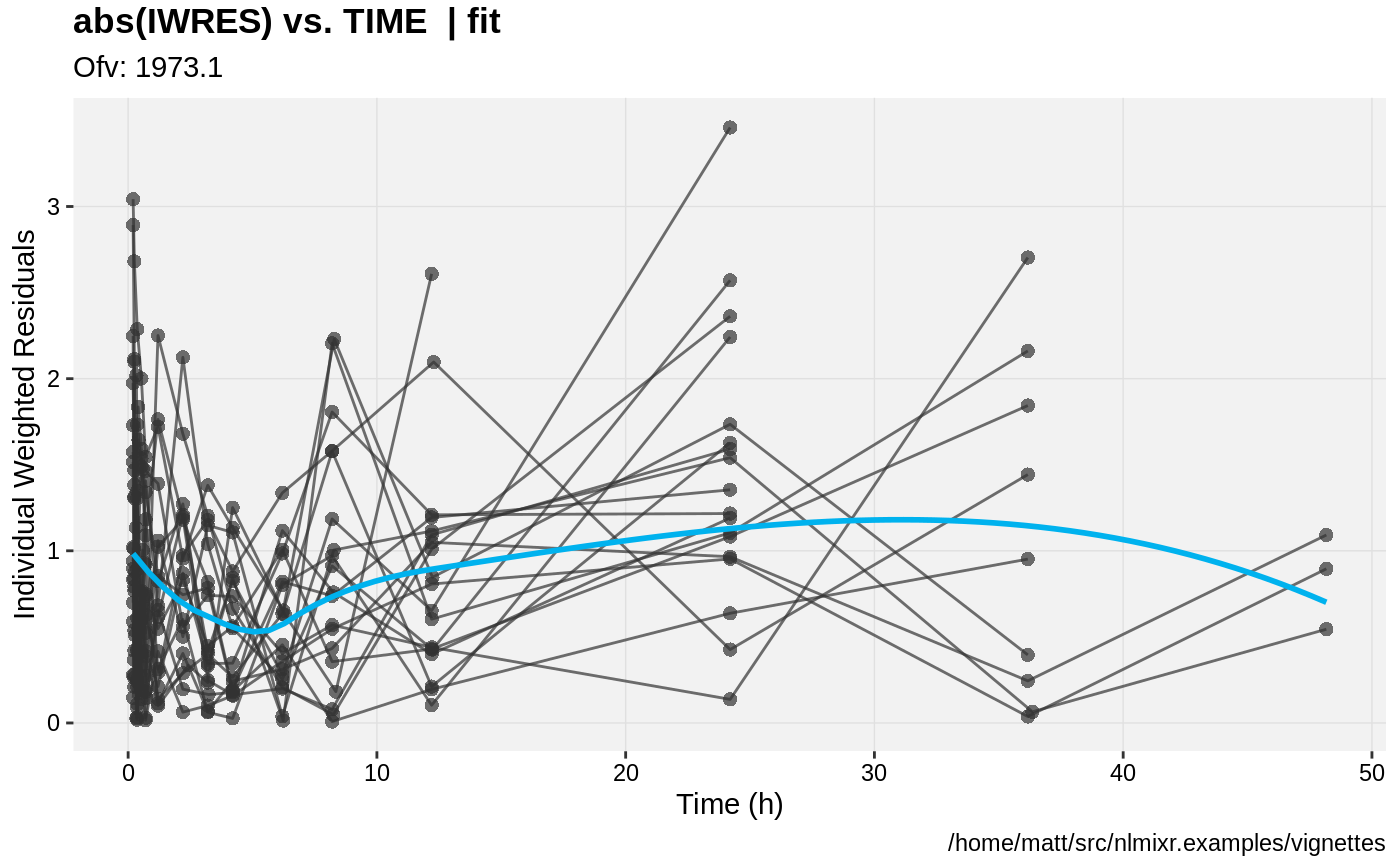
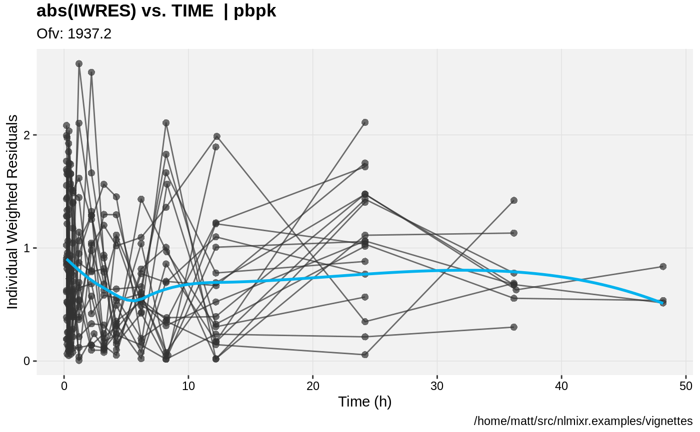
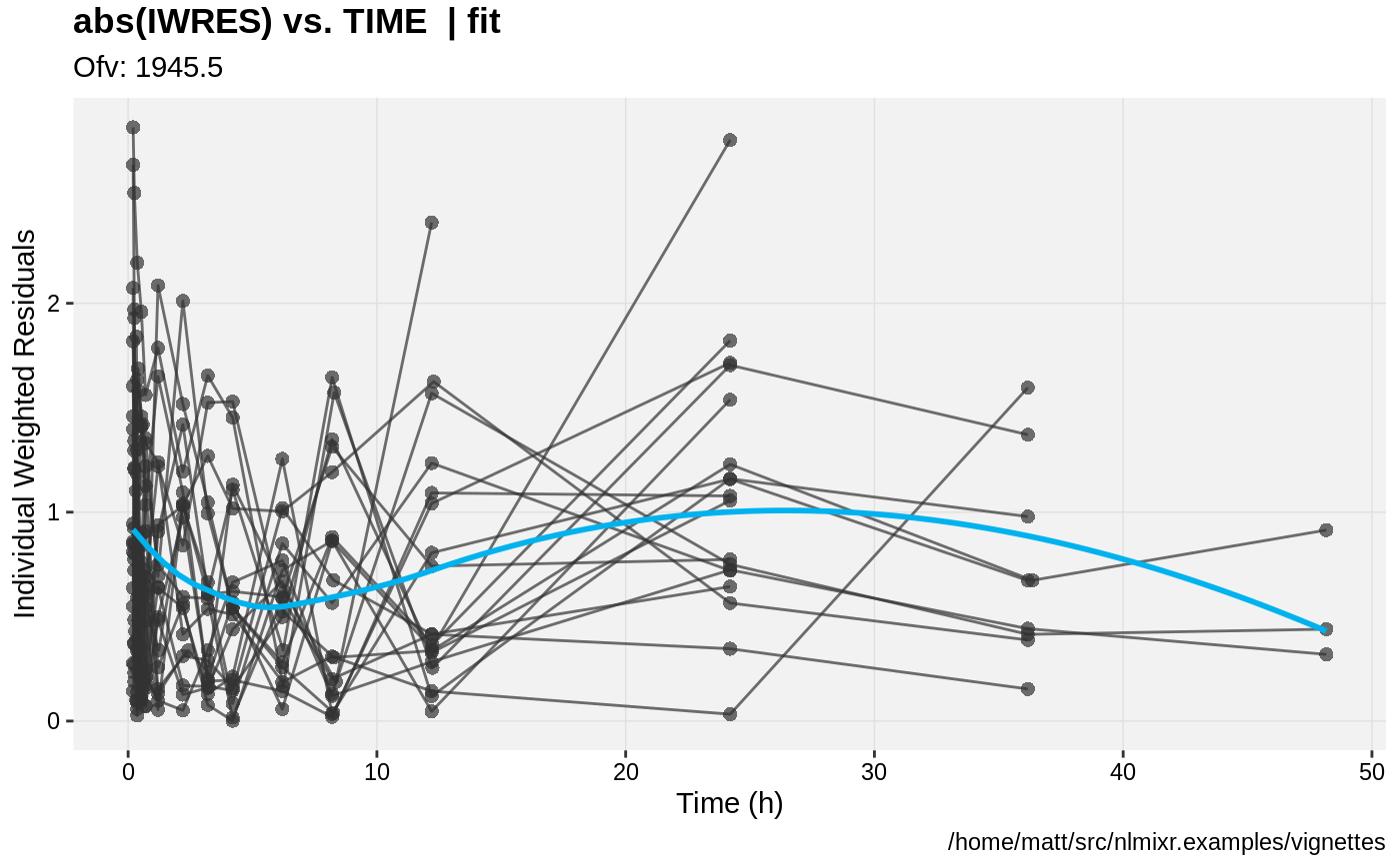
    print(absval_res_vs_idv(xpdb, res = 'IWRES') +
          ylab("Individual Weighted Residuals") +
          xlab("Time (h)"))

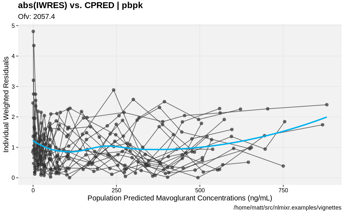
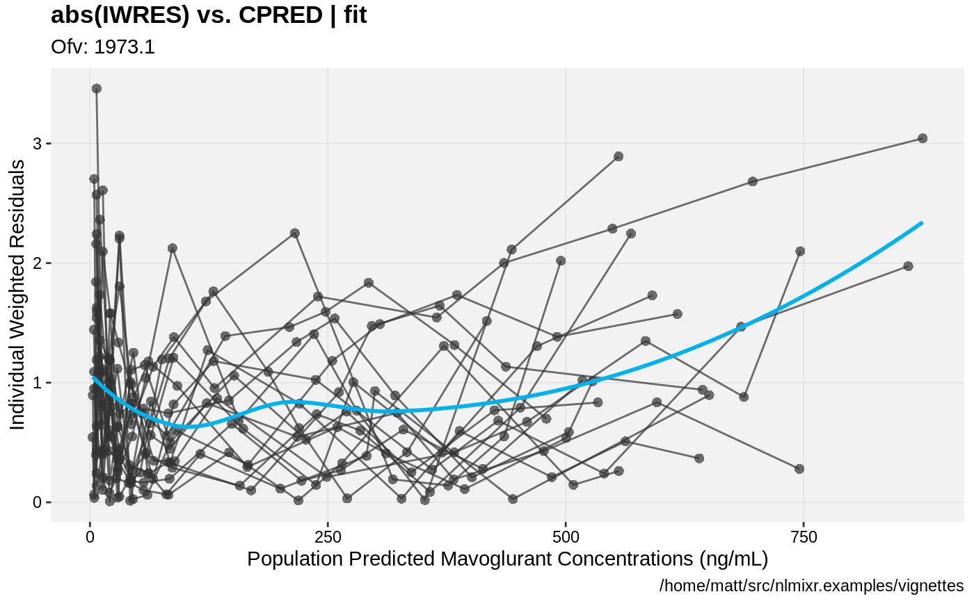
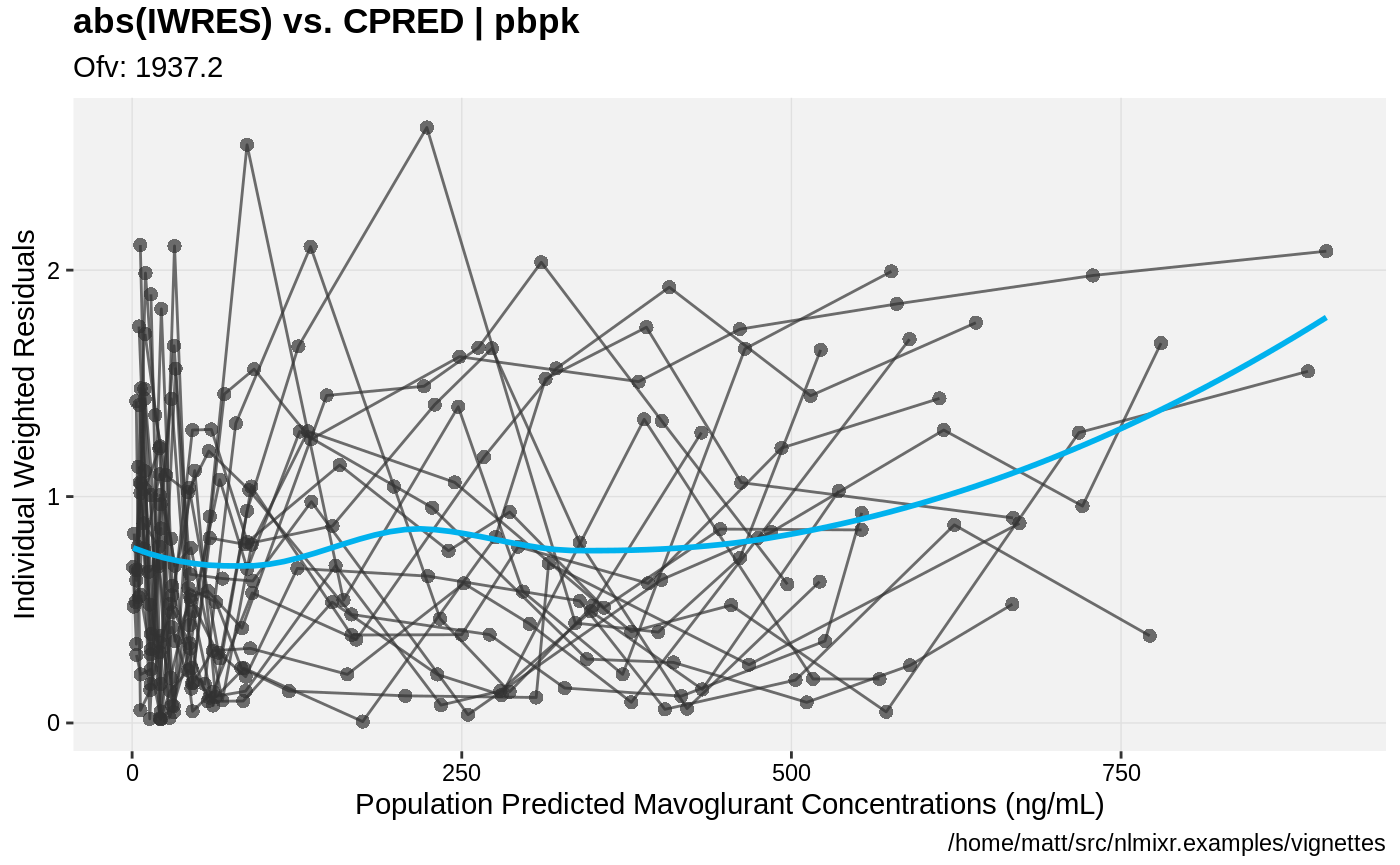
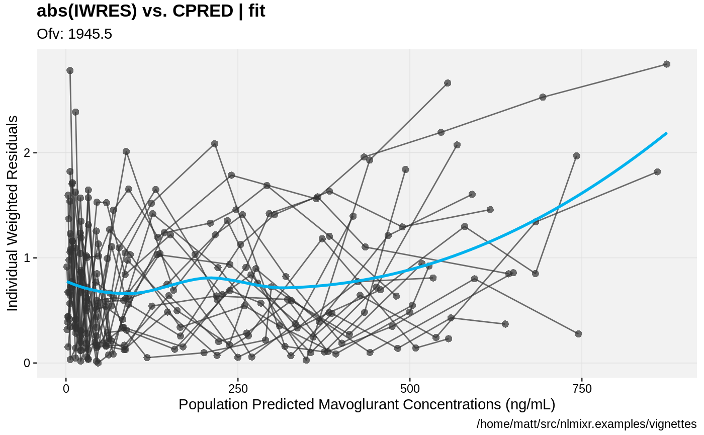
    print(absval_res_vs_pred(xpdb, res = 'IWRES') +
          ylab("Individual Weighted Residuals") +
          xlab("Population Predicted Mavoglurant Concentrations (ng/mL)"))

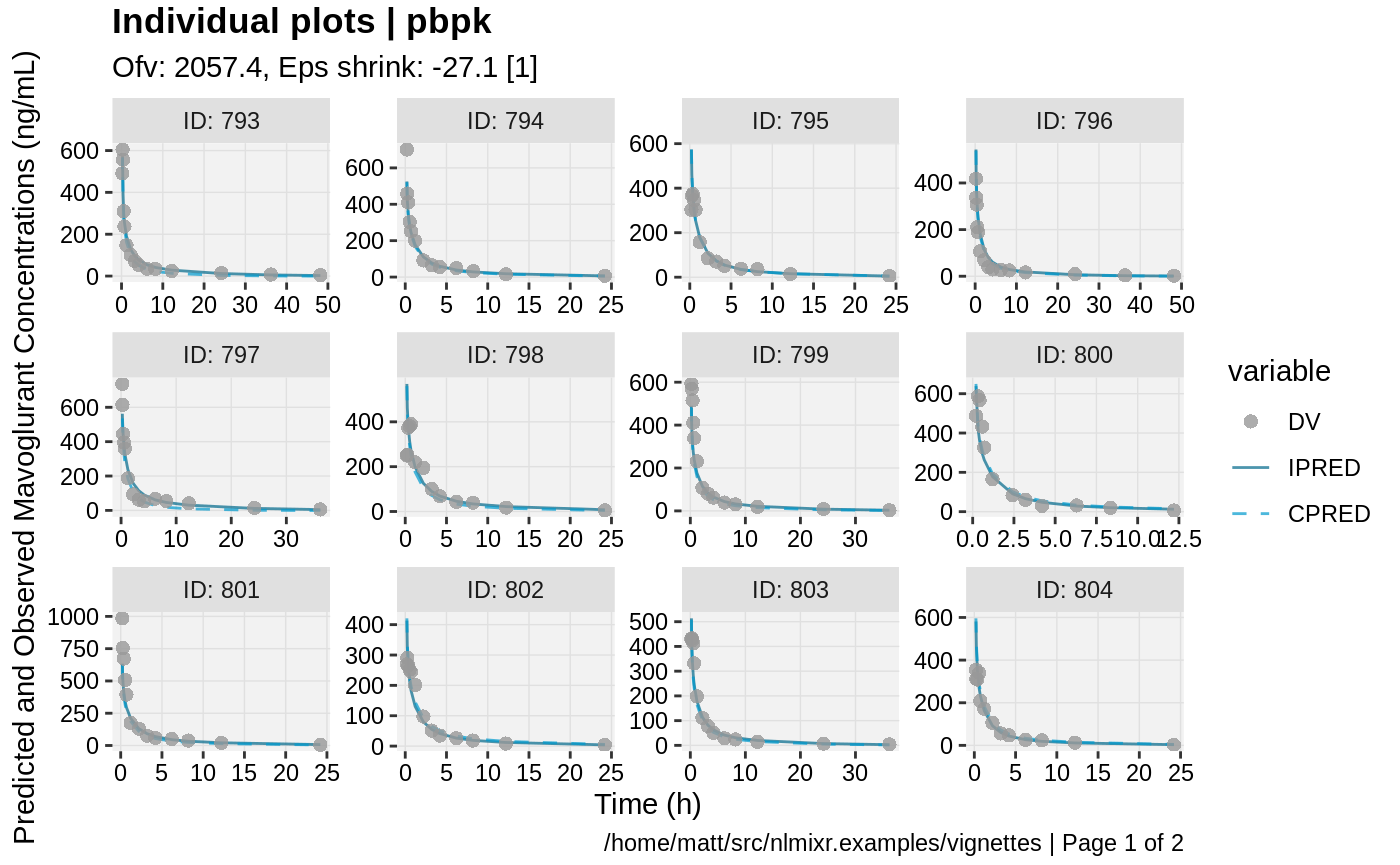
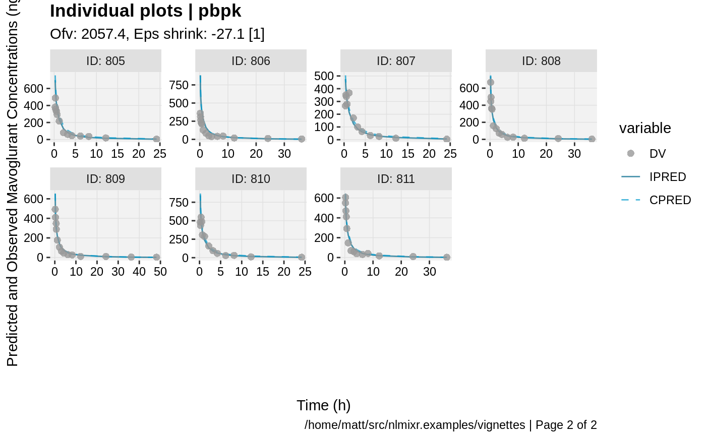
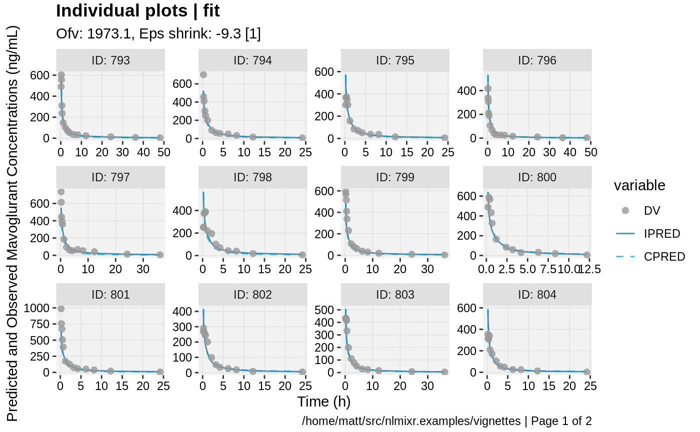
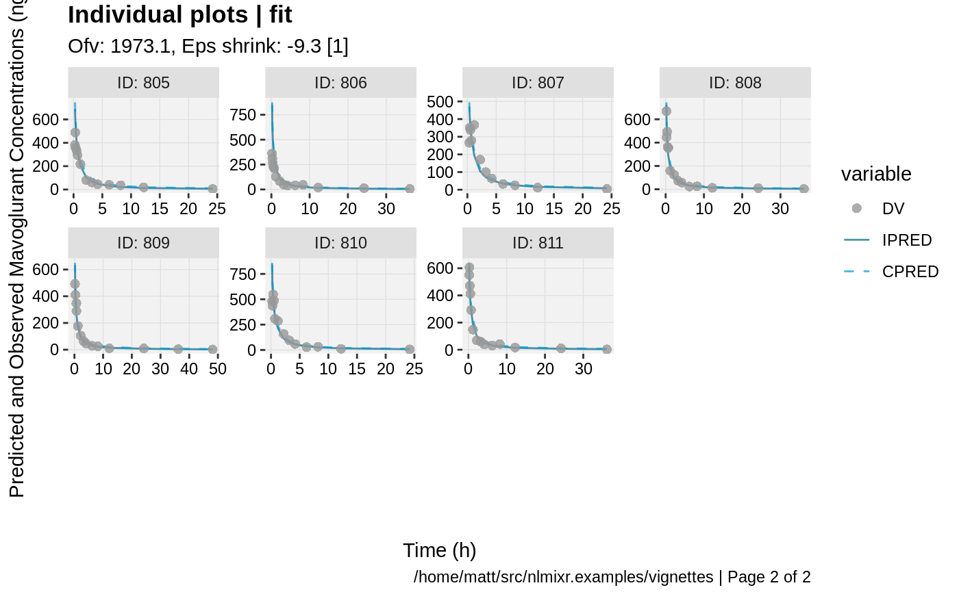
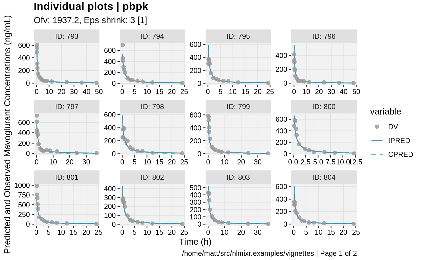
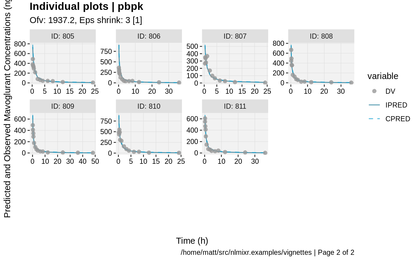
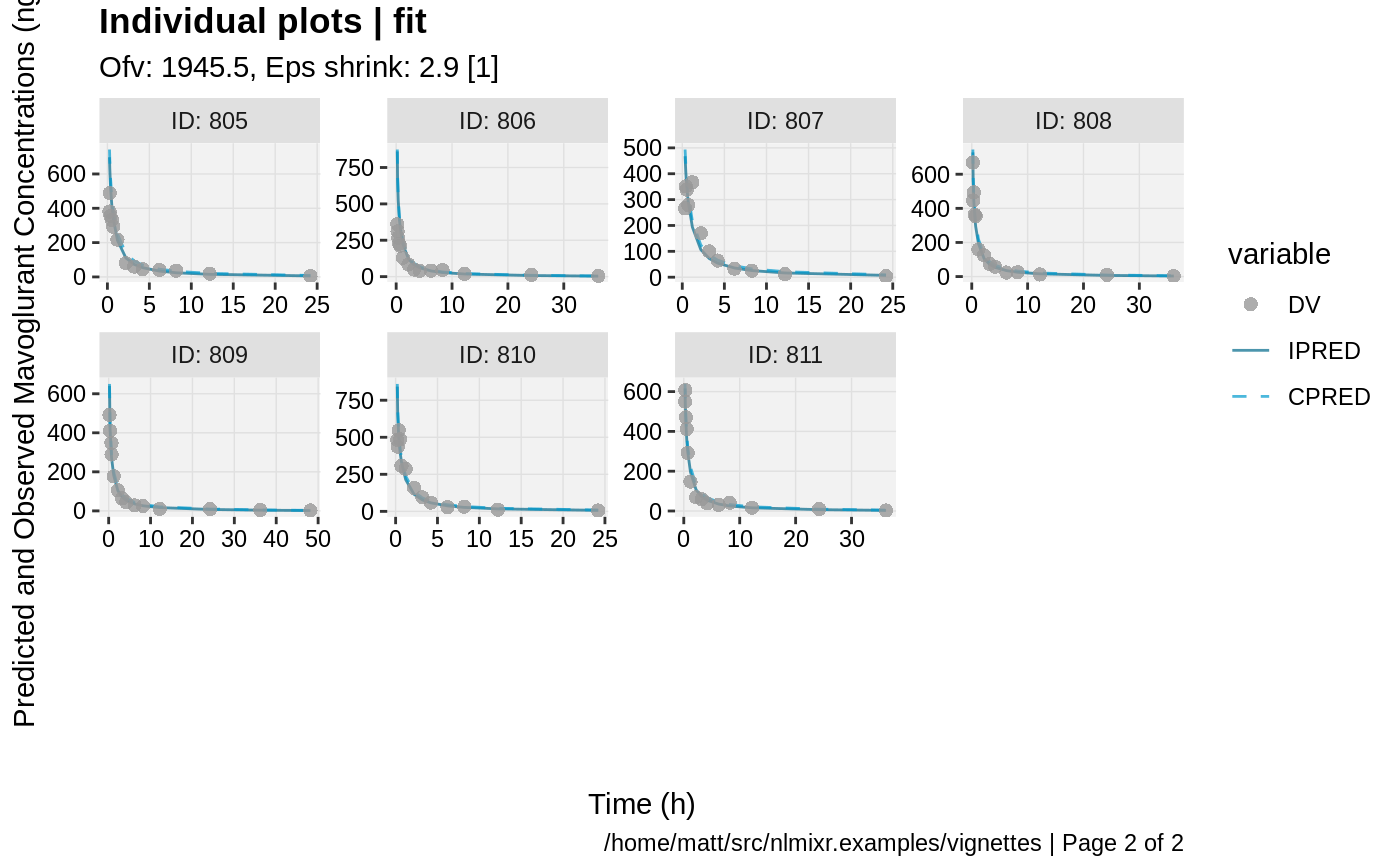
    print(ind_plots(xpdb, nrow=3, ncol=4) +
          ylab("Predicted and Observed Mavoglurant Concentrations (ng/mL)") +
          xlab("Time (h)"))

    print(res_distrib(xpdb) +
          ylab("Density") +
          xlab("Conditional Weighted Residuals"));
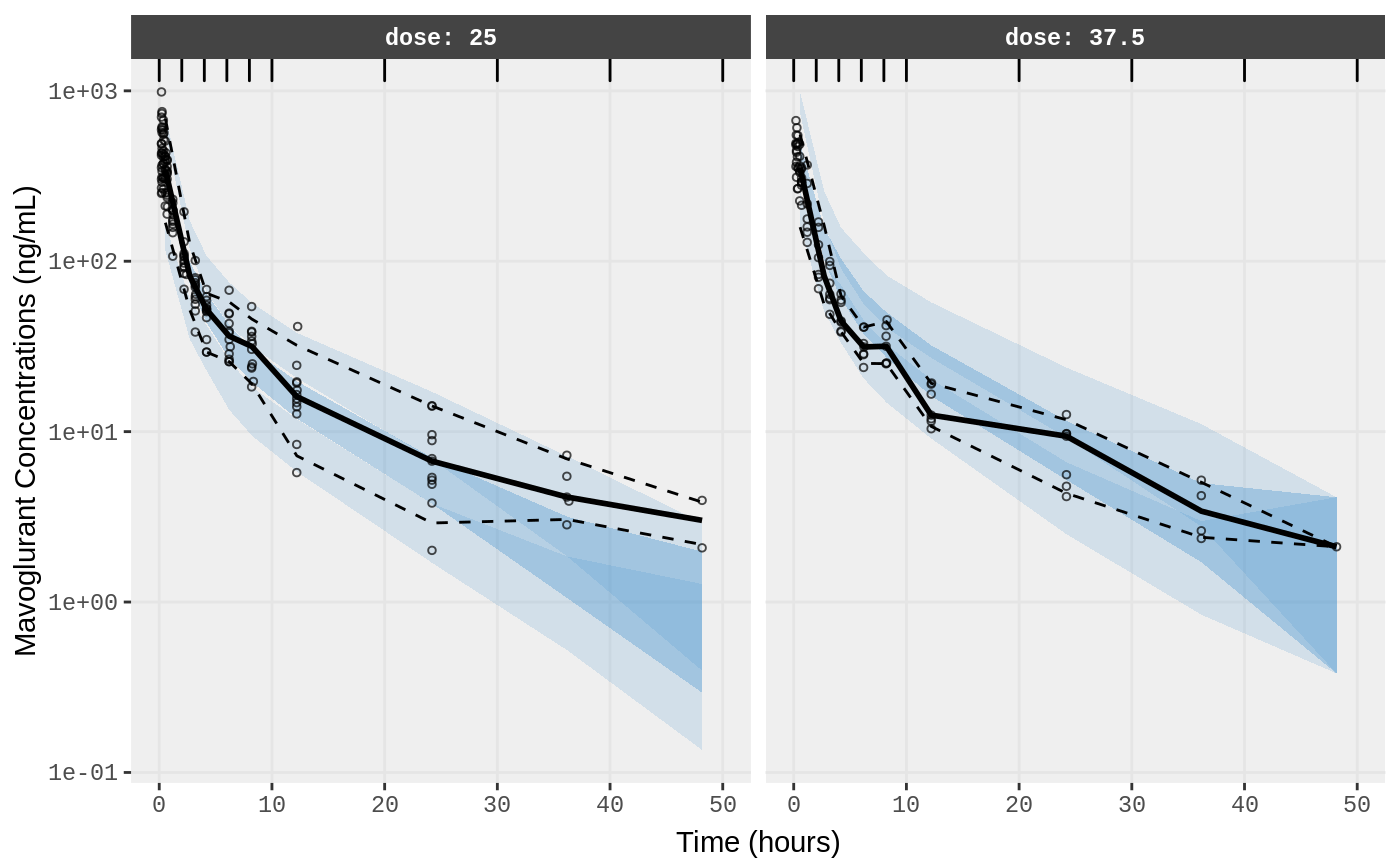
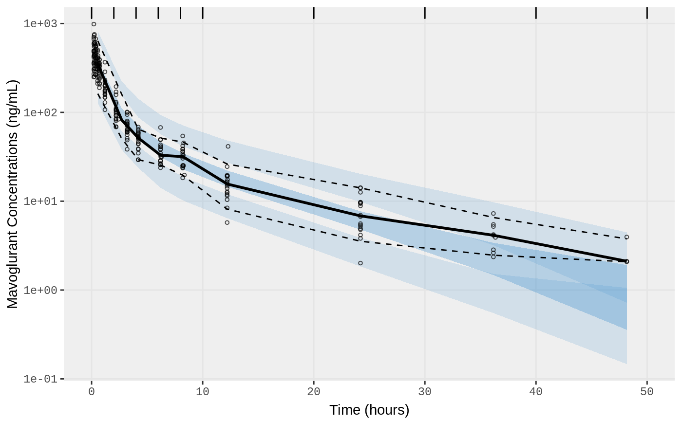
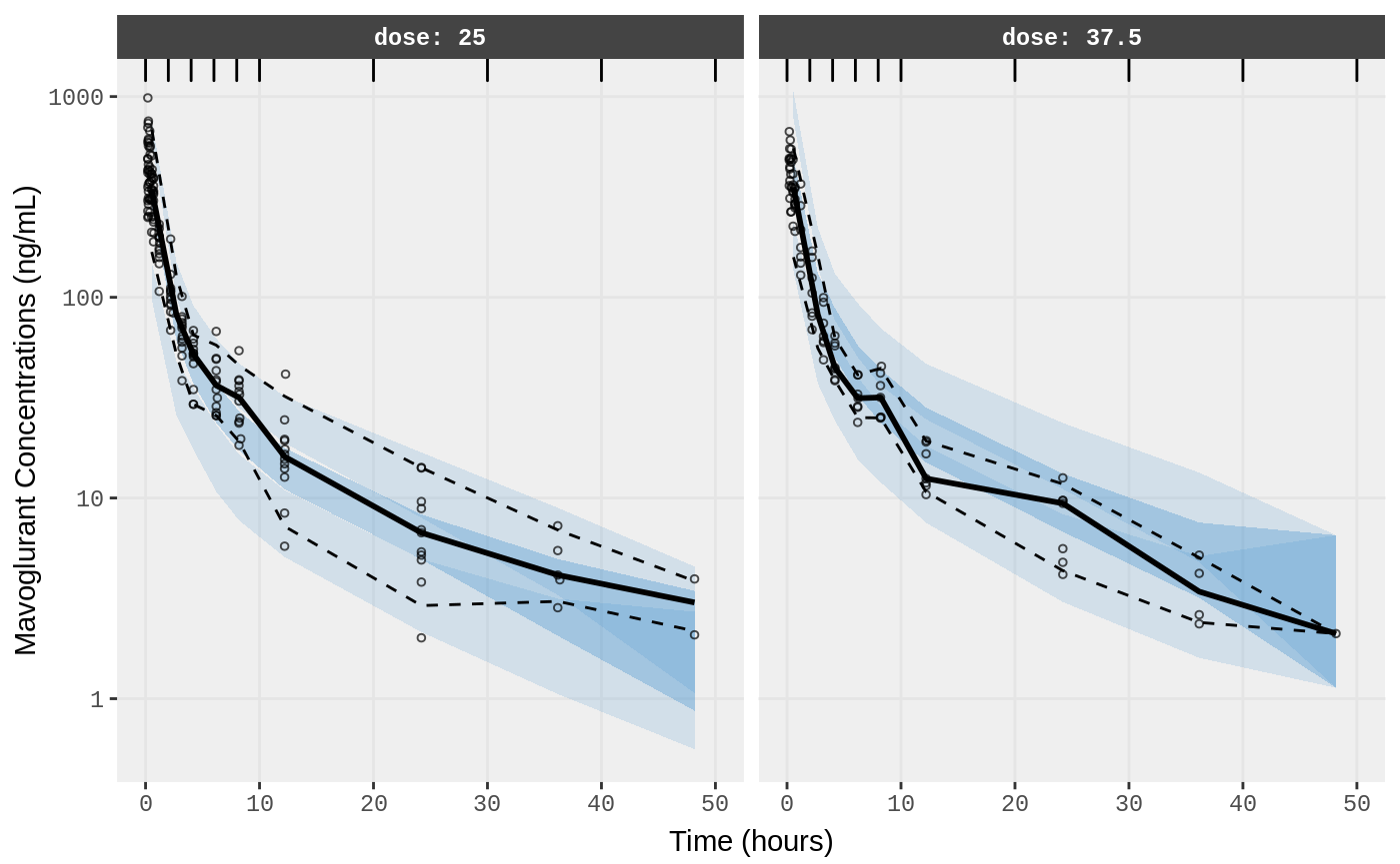
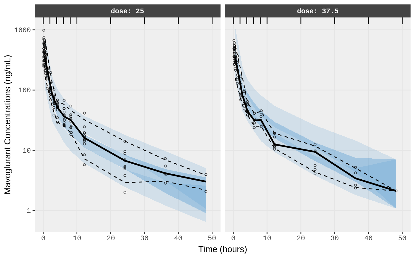
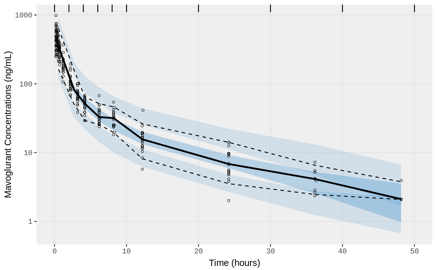
    ##Visual Predictive Checks
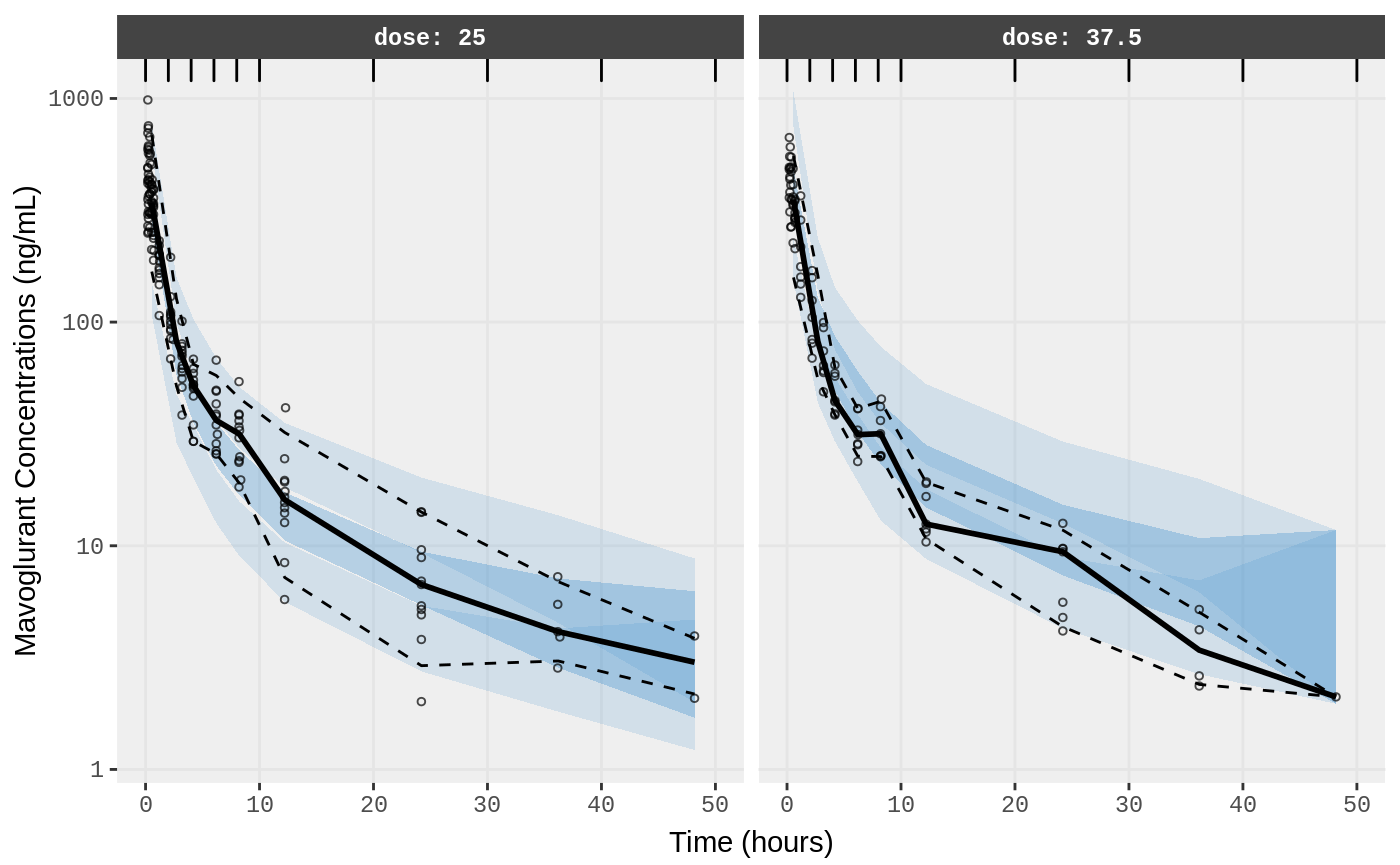
    f1 <- vpc.ui(fit,n=500,stratify=c("dose"), show=list(obs_dv=T), log_y=TRUE,
           bins = c(0, 2, 4, 6, 8, 10, 20, 30, 40, 50),
           ylab = "Mavoglurant Concentrations (ng/mL)",
           xlab = "Time (hours)")
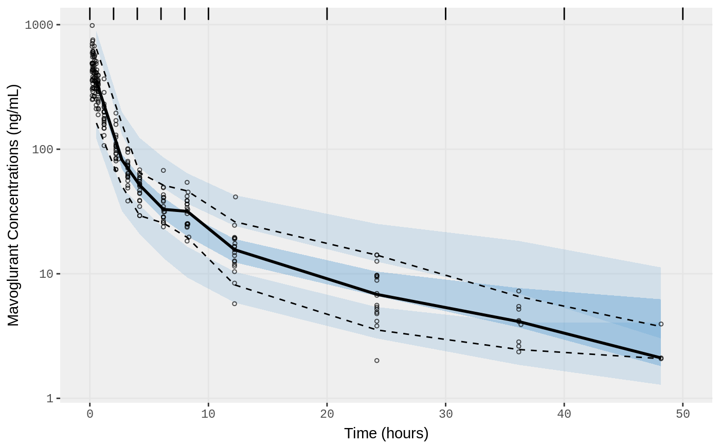
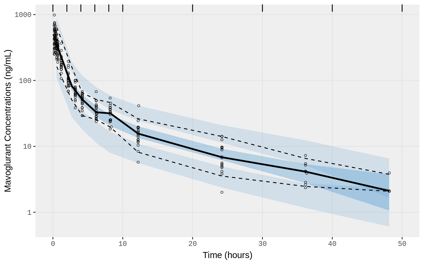
    f2 <- vpc.ui(fit,n=500, show=list(obs_dv=T), bins = c(0, 2, 4, 6, 8, 10, 20, 30, 40, 50), log_y=TRUE,
                 ylab = "Mavoglurant Concentrations (ng/mL)", xlab = "Time (hours)")
    plot(f1)
    plot(f2)
}

SAEM

Fit add+prop SAEM

fit.addProp.S <- nlmixr(pbpk, dat, est="saem", table=list(cwres=TRUE, npde=TRUE))
#> Loading model already run (/tmp/RtmpXKdUFj/temp_libpath58be457a881a/nlmixr.examples/nlmixr-pbpk-dat-saem-699583adb0bac0c648b4790d4c6c6ae6.rds)
#> Warning in lapply(X = X, FUN = FUN, ...): ID missing in parameters dataset;
#>  Parameters are assumed to have the same order as the IDs in the event dataset

gofs(fit.addProp.S);
#> Warning: `complete_()` is deprecated as of tidyr 1.0.0.
#> Please use `complete()` instead.
#> This warning is displayed once per session.
#> Call `lifecycle::last_warnings()` to see where this warning was generated.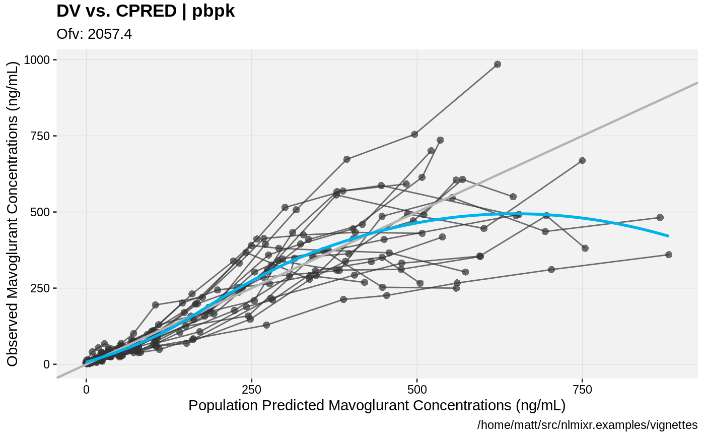

#> Loading vpc already run (/tmp/RtmpXKdUFj/temp_libpath58be457a881a/nlmixr.examples/nlmixr-vpc-pbpk-dat--1b40dbdb827d297602b0fce99e4f35f5.rds)
#> Loading vpc already run (/tmp/RtmpXKdUFj/temp_libpath58be457a881a/nlmixr.examples/nlmixr-vpc-pbpk-dat--119a36afbe069fea277d7a7b784558cf.rds)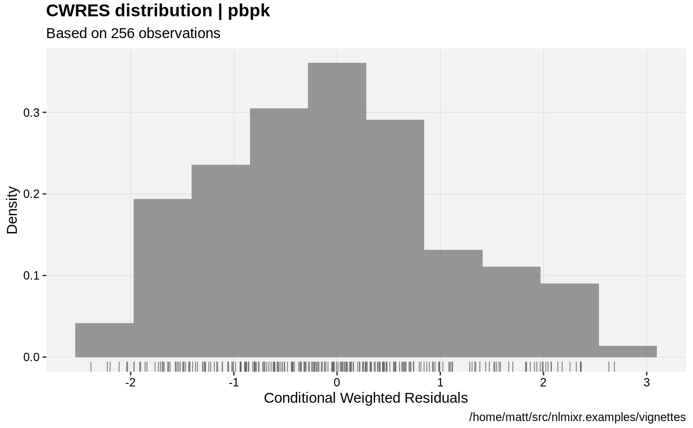

Change error to lognormal

fit.lnorm.S <- pbpk %>%
    model({C15 ~ lnorm(lnorm.err)}) %>% # Change C15 to be log-normally distributed
    ## Requires data since piping from pbpk model
    nlmixr(dat,est="saem", table=list(cwres=TRUE, npde=TRUE))
#> Loading model already run (/tmp/RtmpXKdUFj/temp_libpath58be457a881a/nlmixr.examples/nlmixr-saem-9570ef3429e09e1bdbd76e4b0fb7af69.rds)
#> Warning in lapply(X = X, FUN = FUN, ...): ID missing in parameters dataset;
#>  Parameters are assumed to have the same order as the IDs in the event dataset

NOTE: lognormal distribution AIC/loglik/etc is on normal scale. Therefore, you can compare the AICs between fit.lnorm and fit.addProp since they are calculated on the same scale.

In this case you can see that the AIC for the log-normal model is better than the AIC for the addProp model.

gofs(fit.lnorm.S);

#> Loading vpc already run (/tmp/RtmpXKdUFj/temp_libpath58be457a881a/nlmixr.examples/nlmixr-vpc--584acd366a954b1ade6d444347b5f89f.rds)
#> Loading vpc already run (/tmp/RtmpXKdUFj/temp_libpath58be457a881a/nlmixr.examples/nlmixr-vpc--8a1b72792363c5c8a00b55dc589793fa.rds)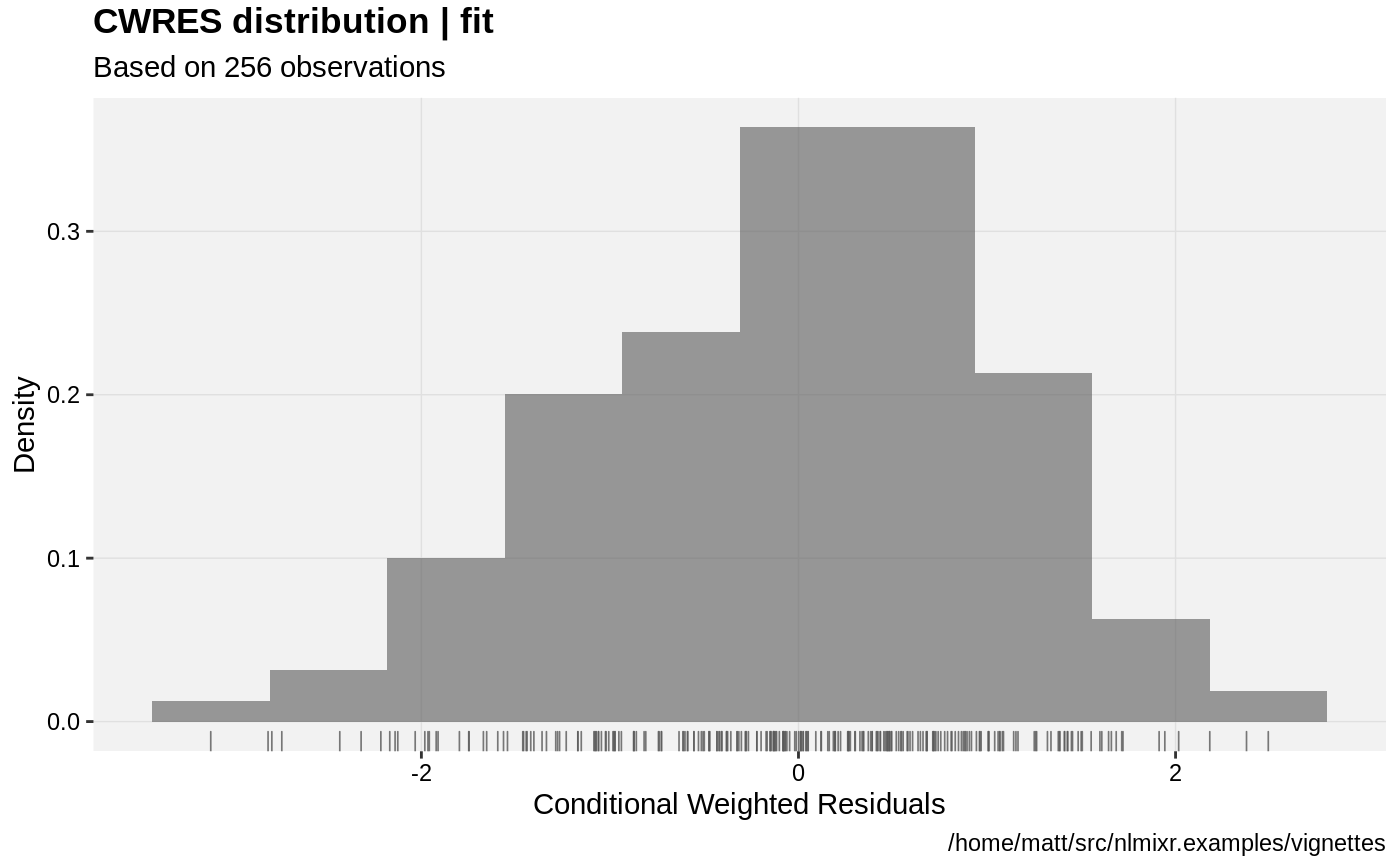

Piping to FOCEi

You can pipe models from different estimation methods to new estimation methods.

Additive + Proportional

fit.addProp.F <- fit.addProp.S %>%
    nlmixr(est="focei", table=list(cwres=TRUE, npde=TRUE));
#> Loading model already run (/tmp/RtmpXKdUFj/temp_libpath58be457a881a/nlmixr.examples/nlmixr-pbpk-dat-focei-c4d353e3425a7b7c59f2f749be162825.rds)
#> Warning in lapply(X = X, FUN = FUN, ...): ID missing in parameters dataset;
#>  Parameters are assumed to have the same order as the IDs in the event dataset
#> Warning in lapply(X = X, FUN = FUN, ...): Initial ETAs were nudged; (Can
#> control by foceiControl(etaNudge=.))
#> Warning in lapply(X = X, FUN = FUN, ...): ETAs were reset to zero during
#> optimization; (Can control by foceiControl(resetEtaP=.))
#> Warning in lapply(X = X, FUN = FUN, ...): Gradient problems with initial
#> estimate and covariance; see $scaleInfo
## Since this was a model pipline, the data
## remains the same as the last fit.

gofs(fit.addProp.F);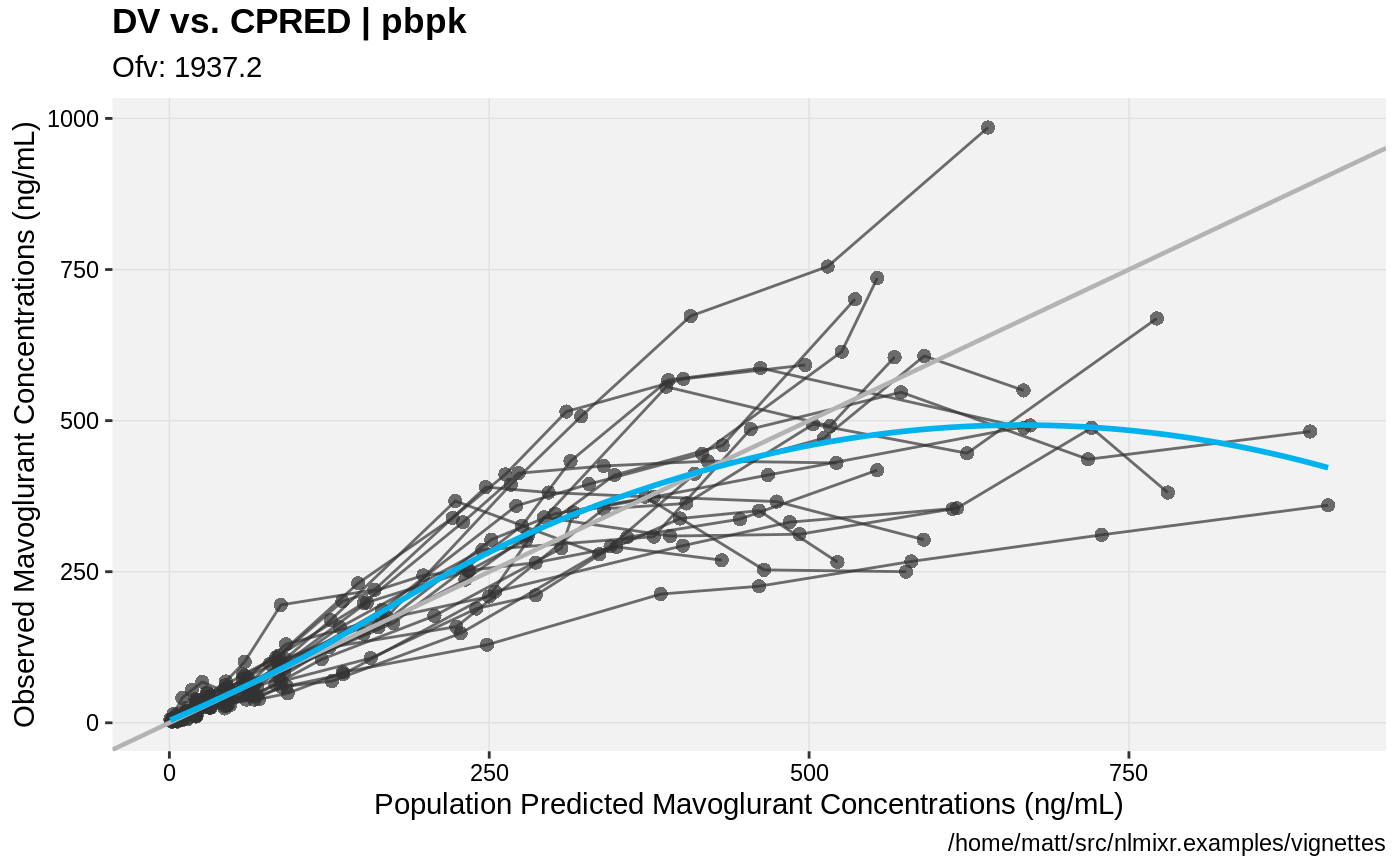

#> Loading vpc already run (/tmp/RtmpXKdUFj/temp_libpath58be457a881a/nlmixr.examples/nlmixr-vpc-pbpk-dat--ebb9ebd29f5f84acdaa1034c58c88f11.rds)
#> Loading vpc already run (/tmp/RtmpXKdUFj/temp_libpath58be457a881a/nlmixr.examples/nlmixr-vpc-pbpk-dat--4a83accb8ed983ad01aec28903a69e34.rds)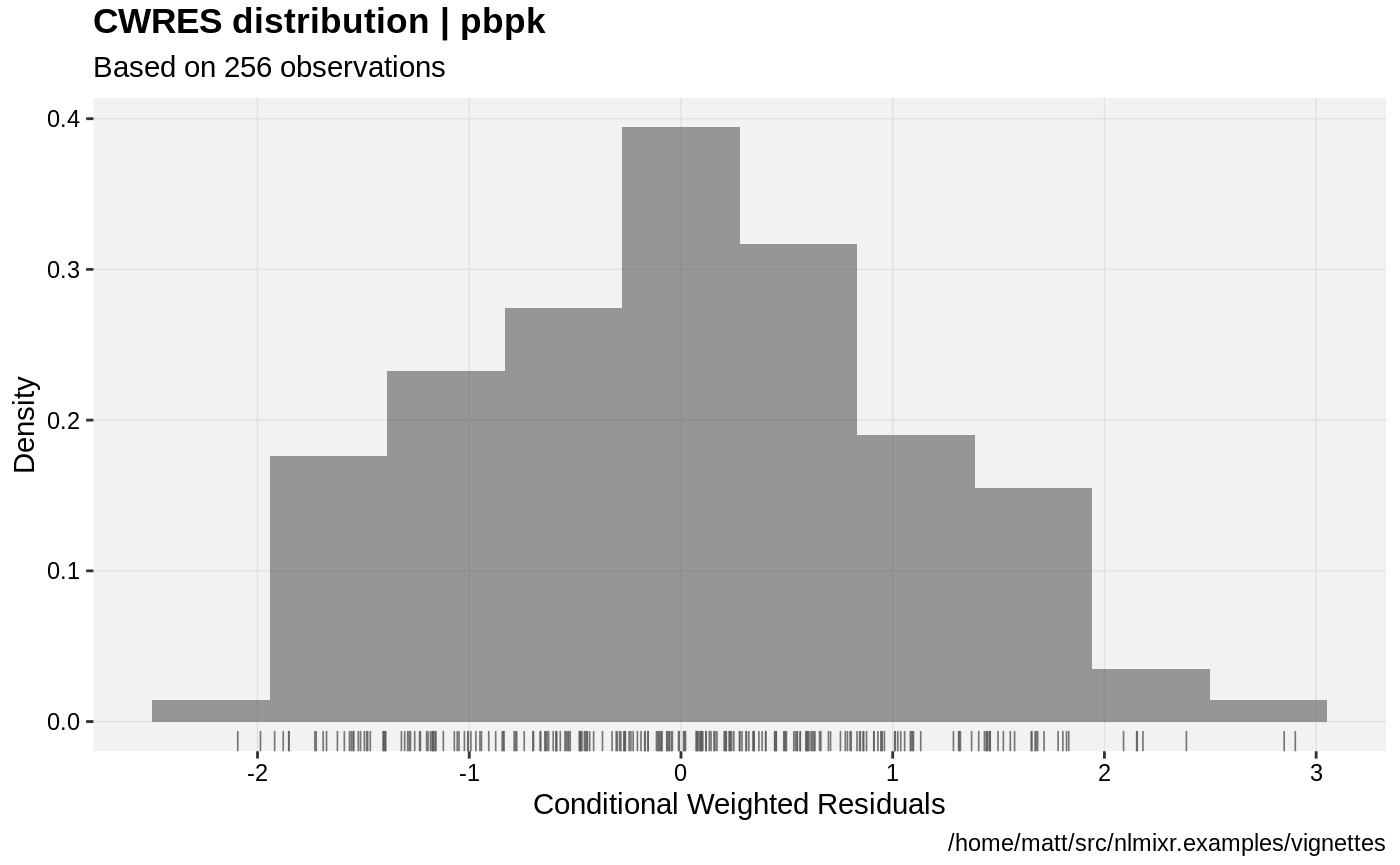

Lognoral

fit.lnorm.F <- fit.addProp.F %>%
    model({C15 ~ lnorm(lnorm.err)}) %>%
    nlmixr(est="focei", table=list(cwres=TRUE, npde=TRUE));
#> Loading model already run (/tmp/RtmpXKdUFj/temp_libpath58be457a881a/nlmixr.examples/nlmixr-focei-6220db148acc28521ed91be821211b1e.rds)
#> Warning in lapply(X = X, FUN = FUN, ...): ID missing in parameters dataset;
#>  Parameters are assumed to have the same order as the IDs in the event dataset
#> Warning in lapply(X = X, FUN = FUN, ...): Initial ETAs were nudged; (Can
#> control by foceiControl(etaNudge=.))
#> Warning in lapply(X = X, FUN = FUN, ...): ETAs were reset to zero during
#> optimization; (Can control by foceiControl(resetEtaP=.))
#> Warning in lapply(X = X, FUN = FUN, ...): Gradient problems with initial
#> estimate and covariance; see $scaleInfo
## In this model pipline we are changing the fit method to focei.

gofs(fit.lnorm.F);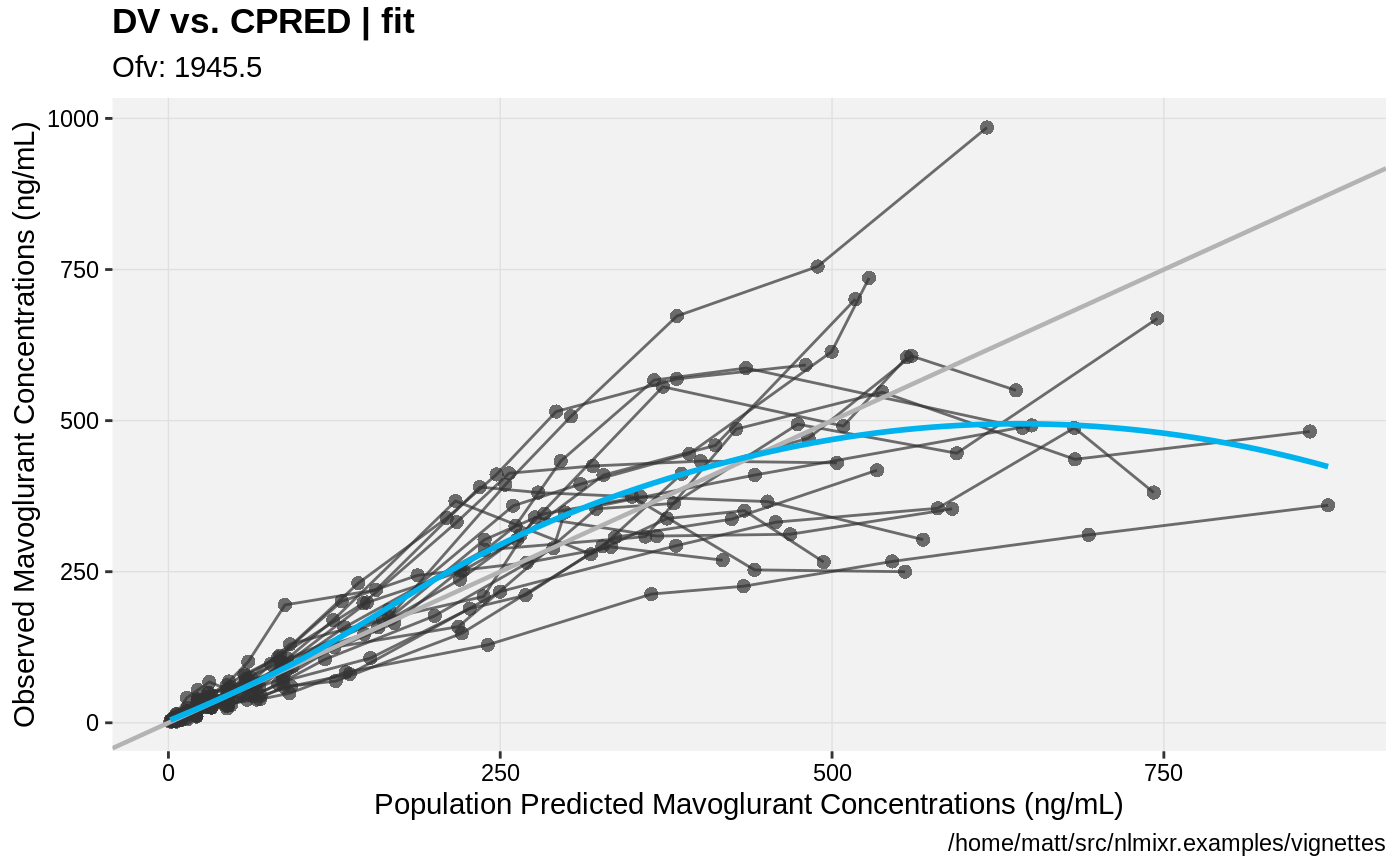

#> Loading vpc already run (/tmp/RtmpXKdUFj/temp_libpath58be457a881a/nlmixr.examples/nlmixr-vpc--9eb12e1c9cae6478af6d9a2689720c3a.rds)
#> Loading vpc already run (/tmp/RtmpXKdUFj/temp_libpath58be457a881a/nlmixr.examples/nlmixr-vpc--de1ad949829fa584a7318449ec45ad5d.rds)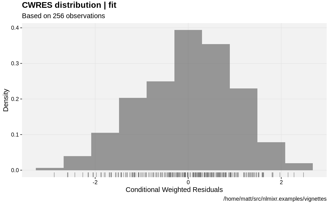

# Traditional lognormal estimates are identical

datL  <- dat
datL$DV <- log(datL$DV);

pbpkL <- function(){
    ini({
        ##theta=exp(c(1.1, .3, 2, 7.6, .003, .3))
        lKbBR = 1.1
        lKbMU = 0.3
        lKbAD = 2
        lCLint = 7.6
        lKbBO = 0.03
        lKbRB = 0.3
        eta.LClint ~ 4
        add.err <- 1
    })
    model({
        KbBR = exp(lKbBR)
        KbMU = exp(lKbMU)
        KbAD = exp(lKbAD)
        CLint= exp(lCLint + eta.LClint)
        KbBO = exp(lKbBO)
        KbRB = exp(lKbRB)

        ## Regional blood flows
        CO  = (187.00*WT^0.81)*60/1000;         # Cardiac output (L/h) from White et al (1968)
        QHT = 4.0 *CO/100;
        QBR = 12.0*CO/100;
        QMU = 17.0*CO/100;
        QAD = 5.0 *CO/100;
        QSK = 5.0 *CO/100;
        QSP = 3.0 *CO/100;
        QPA = 1.0 *CO/100;
        QLI = 25.5*CO/100;
        QST = 1.0 *CO/100;
        QGU = 14.0*CO/100;
        QHA = QLI - (QSP + QPA + QST + QGU); # Hepatic artery blood flow
        QBO = 5.0 *CO/100;
        QKI = 19.0*CO/100;
        QRB = CO - (QHT + QBR + QMU + QAD + QSK + QLI + QBO + QKI);
        QLU = QHT + QBR + QMU + QAD + QSK + QLI + QBO + QKI + QRB;

        ## Organs' volumes = organs' weights / organs' density
        VLU = (0.76 *WT/100)/1.051;
        VHT = (0.47 *WT/100)/1.030;
        VBR = (2.00 *WT/100)/1.036;
        VMU = (40.00*WT/100)/1.041;
        VAD = (21.42*WT/100)/0.916;
        VSK = (3.71 *WT/100)/1.116;
        VSP = (0.26 *WT/100)/1.054;
        VPA = (0.14 *WT/100)/1.045;
        VLI = (2.57 *WT/100)/1.040;
        VST = (0.21 *WT/100)/1.050;
        VGU = (1.44 *WT/100)/1.043;
        VBO = (14.29*WT/100)/1.990;
        VKI = (0.44 *WT/100)/1.050;
        VAB = (2.81 *WT/100)/1.040;
        VVB = (5.62 *WT/100)/1.040;
        VRB = (3.86 *WT/100)/1.040;

        ## Fixed parameters
        BP = 0.61;      # Blood:plasma partition coefficient
        fup = 0.028;    # Fraction unbound in plasma
        fub = fup/BP;   # Fraction unbound in blood

        KbLU = exp(0.8334);
        KbHT = exp(1.1205);
        KbSK = exp(-.5238);
        KbSP = exp(0.3224);
        KbPA = exp(0.3224);
        KbLI = exp(1.7604);
        KbST = exp(0.3224);
        KbGU = exp(1.2026);
        KbKI = exp(1.3171);

        ##-----------------------------------------
        S15 = VVB*BP/1000;
        C15 = Venous_Blood/S15
        lnC15 = log(C15);

        ##-----------------------------------------
        d/dt(Lungs) = QLU*(Venous_Blood/VVB - Lungs/KbLU/VLU);
        d/dt(Heart) = QHT*(Arterial_Blood/VAB - Heart/KbHT/VHT);
        d/dt(Brain) = QBR*(Arterial_Blood/VAB - Brain/KbBR/VBR);
        d/dt(Muscles) = QMU*(Arterial_Blood/VAB - Muscles/KbMU/VMU);
        d/dt(Adipose) = QAD*(Arterial_Blood/VAB - Adipose/KbAD/VAD);
        d/dt(Skin) = QSK*(Arterial_Blood/VAB - Skin/KbSK/VSK);
        d/dt(Spleen) = QSP*(Arterial_Blood/VAB - Spleen/KbSP/VSP);
        d/dt(Pancreas) = QPA*(Arterial_Blood/VAB - Pancreas/KbPA/VPA);
        d/dt(Liver) = QHA*Arterial_Blood/VAB + QSP*Spleen/KbSP/VSP + QPA*Pancreas/KbPA/VPA + QST*Stomach/KbST/VST + QGU*Gut/KbGU/VGU - CLint*fub*Liver/KbLI/VLI - QLI*Liver/KbLI/VLI;
        d/dt(Stomach) = QST*(Arterial_Blood/VAB - Stomach/KbST/VST);
        d/dt(Gut) = QGU*(Arterial_Blood/VAB - Gut/KbGU/VGU);
        d/dt(Bones) = QBO*(Arterial_Blood/VAB - Bones/KbBO/VBO);
        d/dt(Kidneys) = QKI*(Arterial_Blood/VAB - Kidneys/KbKI/VKI);
        d/dt(Arterial_Blood) = QLU*(Lungs/KbLU/VLU - Arterial_Blood/VAB);
        d/dt(Venous_Blood) = QHT*Heart/KbHT/VHT + QBR*Brain/KbBR/VBR +
            QMU*Muscles/KbMU/VMU + QAD*Adipose/KbAD/VAD +
            QSK*Skin/KbSK/VSK + QLI*Liver/KbLI/VLI + QBO*Bones/KbBO/VBO +
            QKI*Kidneys/KbKI/VKI + QRB*Rest_of_Body/KbRB/VRB - QLU*Venous_Blood/VVB;
        d/dt(Rest_of_Body) = QRB*(Arterial_Blood/VAB - Rest_of_Body/KbRB/VRB);

        lnC15 ~ add(add.err)
    })
}

fit.lnorm.trans <- pbpkL %>%
    nlmixr(datL,est="saem", table=list(npde=TRUE, cwres=TRUE))
#> Loading model already run (/tmp/RtmpXKdUFj/temp_libpath58be457a881a/nlmixr.examples/nlmixr-datL-saem-a408e5dbaf1df619264d3b395c892495.rds)
#> Warning in lapply(X = X, FUN = FUN, ...): ID missing in parameters dataset;
#>  Parameters are assumed to have the same order as the IDs in the event dataset

NOTE: the estimates are the same but the AIC is different since it is calculated on the log scale.