Example Model: Phenobarbatol with correlations

2019-10-17

nlmixr

Adding Covariances between random effects

You can simply add co-variances between two random effects by adding the effects together in the model specification block, that is eta.cl+eta.v ~. After that statement, you specify the lower triangular matrix of the fit with c().

An example of this is the Phenobarbital data:

## Load Phenobarb data
library(nlmixr)

Model Specification

pheno <- function() {
  ini({
    tcl <- log(0.008) # typical value of clearance
    tv <-  log(0.6)   # typical value of volume
    ## var(eta.cl)
    eta.cl + eta.v ~ c(1, 
                       0.01, 1) ## cov(eta.cl, eta.v), var(eta.v)
                      # interindividual variability on clearance and volume
    add.err <- 0.1    # residual variability
  })
  model({
    cl <- exp(tcl + eta.cl) # individual value of clearance
    v <- exp(tv + eta.v)    # individual value of volume
    ke <- cl / v            # elimination rate constant
    d/dt(A1) = - ke * A1    # model differential equation
    cp = A1 / v             # concentration in plasma
    cp ~ add(add.err)       # define error model
  })
}

Fit with SAEM

fit <- nlmixr(pheno, pheno_sd, "saem", table=list(cwres=TRUE, npde=TRUE))

print(fit)
#> ── nlmixr SAEM([3mODE[23m); [2m[3mOBJF by FOCEi approximation[23m[22m fit ────────────────────── 
#>           OBJF      AIC      BIC Log-likelihood Condition Number
#> FOCEi 688.6326 985.5036 1003.764      -486.7518         7.536808
#> 
#> ── Time (sec; $time): ───────────────────────────────────────────────────── 
#>            saem    setup table  cwres covariance  npde    other
#> elapsed -31.188 58.27651 0.011 58.296      0.019 0.604 0.918492
#> 
#> ── Population Parameters ($parFixed or $parFixedDf): ────────────────────── 
#>                          Parameter  Est.     SE %RSE
#> tcl     typical value of clearance    -5 0.0752  1.5
#> tv         typical value of volume 0.346 0.0537 15.5
#> add.err       residual variability  2.83            
#>            Back-transformed(95%CI) BSV(CV%) Shrink(SD)%
#> tcl     0.00677 (0.00584, 0.00784)     53.1      1.86% 
#> tv               1.41 (1.27, 1.57)     40.9      1.25% 
#> add.err                       2.83                      
#> 
#>   Covariance Type ($covMethod): linFim
#>   Correlations in between subject variability (BSV) matrix:
#>     cor__eta.v.eta.cl 
#>              0.985   
#> 
#>   Full BSV covariance ($omega) or correlation ($omegaR; diagonals=SDs) 
#>   Distribution stats (mean/skewness/kurtosis/p-value) available in $shrink 
#> 
#> ── Fit Data (object is a modified tibble): ──────────────────────────────── 
#> # A tibble: 155 x 23
#>   ID     TIME    DV  EVID  PRED    RES   WRES IPRED  IRES  IWRES CPRED
#>   <fct> <dbl> <dbl> <int> <dbl>  <dbl>  <dbl> <dbl> <dbl>  <dbl> <dbl>
#> 1 1        2   17.3     0  17.5 -0.228 -0.105  18.5 -1.16 -0.410  17.5
#> 2 1      112.  31       0  27.9  3.10   1.43   29.6  1.37  0.483  27.9
#> 3 2        2    9.7     0  10.5 -0.817 -0.376  12.5 -2.80 -0.989  10.3
#> # … with 152 more rows, and 12 more variables: CRES <dbl>, CWRES <dbl>,
#> #   eta.cl <dbl>, eta.v <dbl>, cl <dbl>, v <dbl>, ke <dbl>, cp <dbl>,
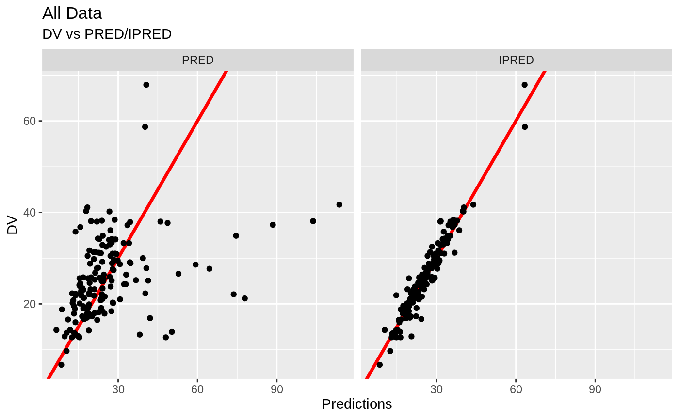
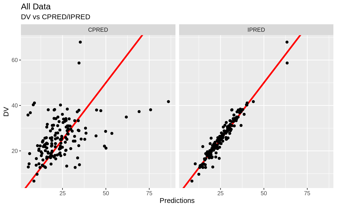
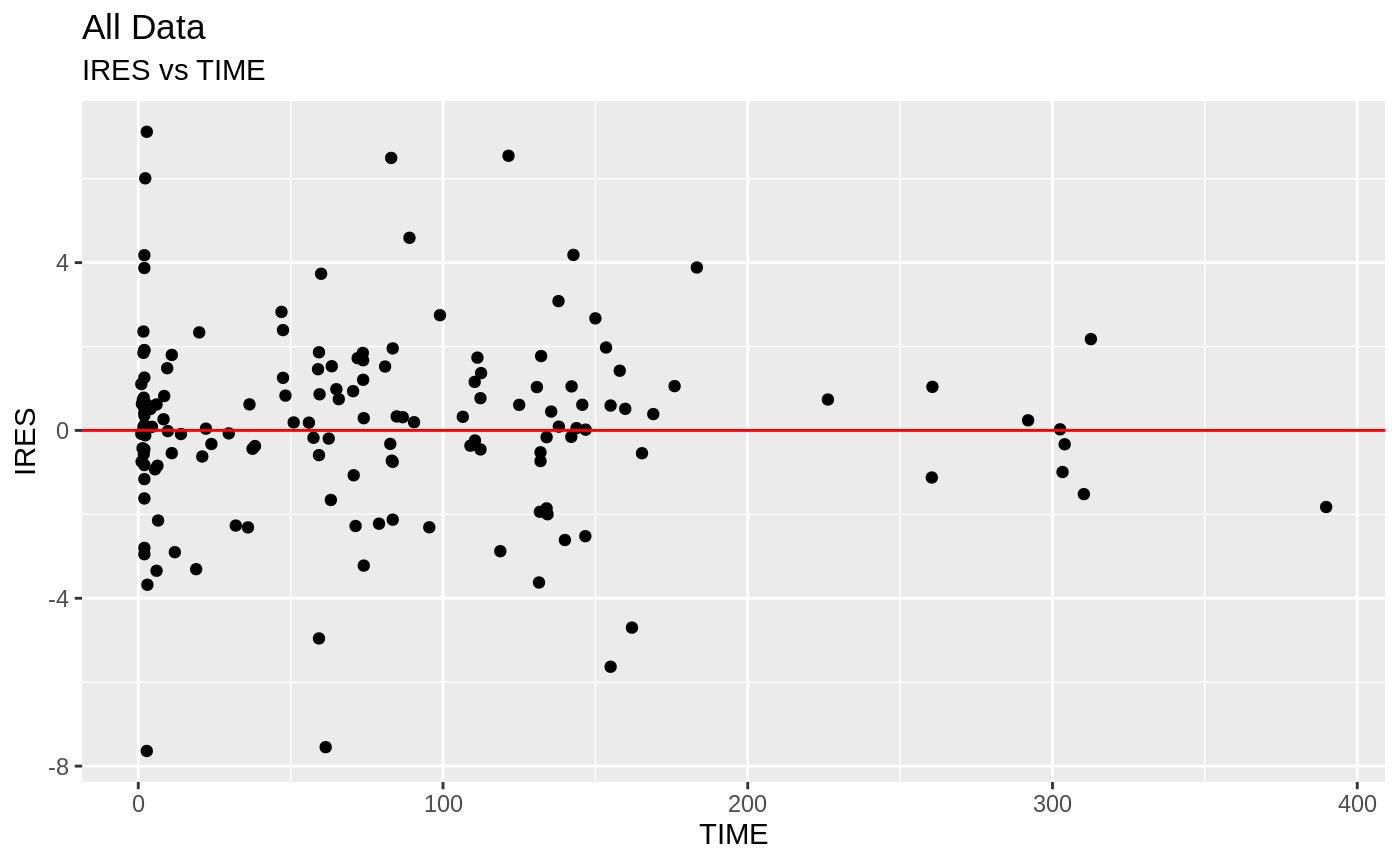
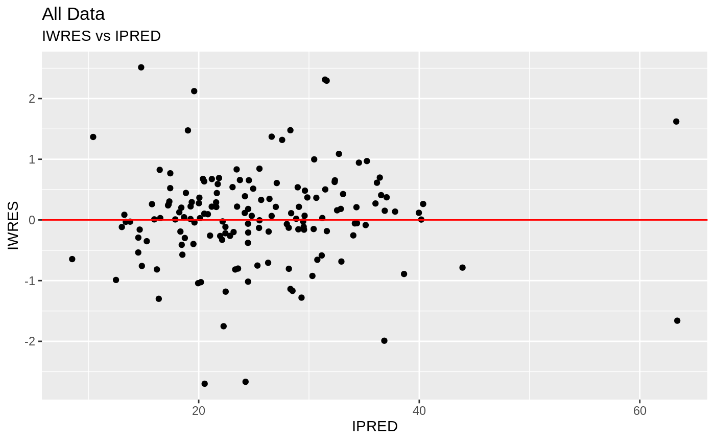
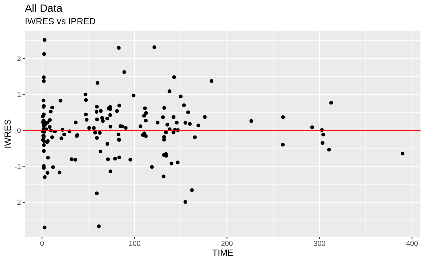
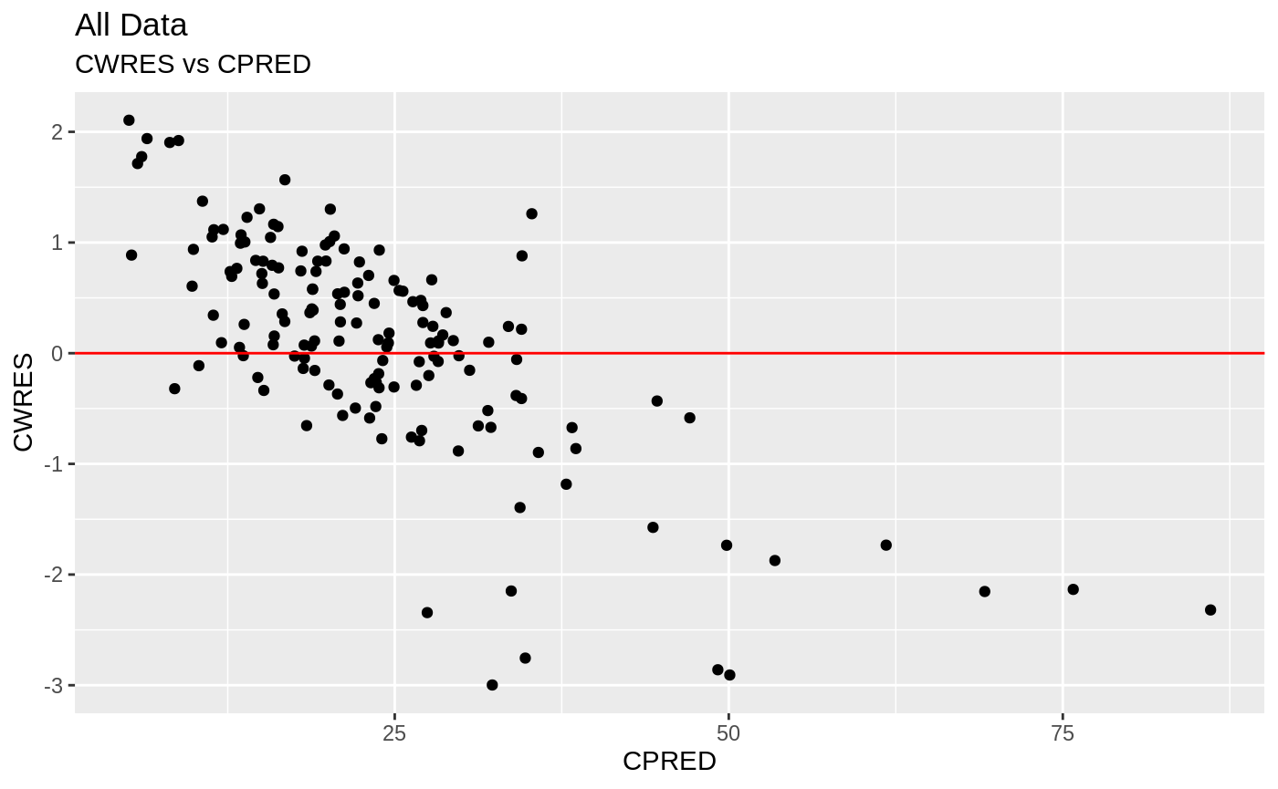
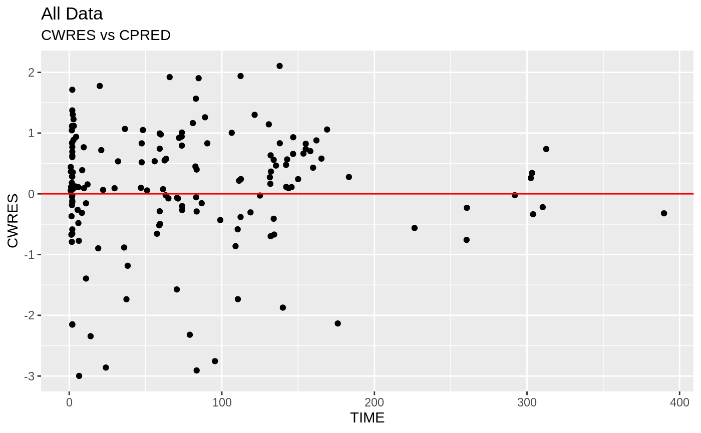
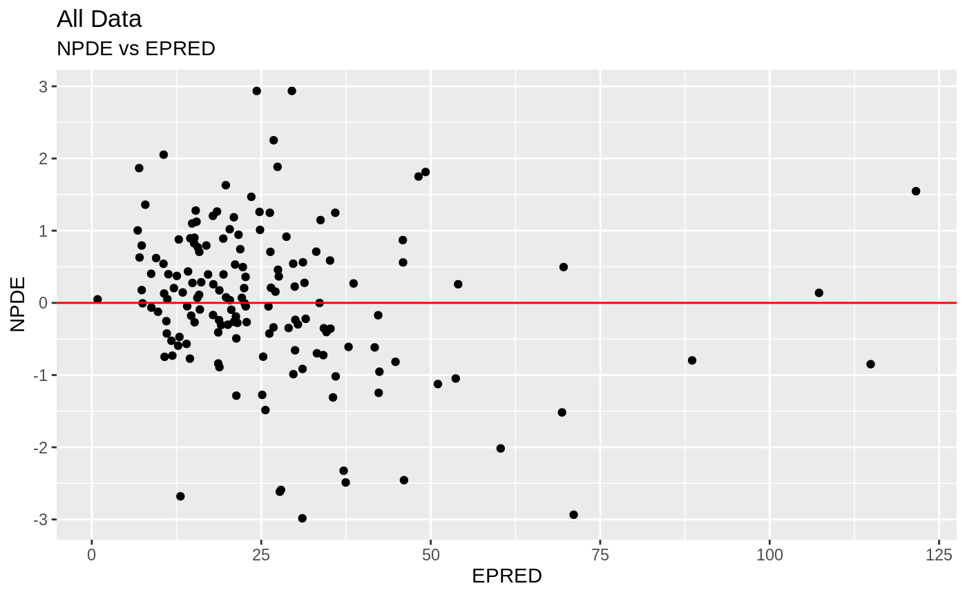
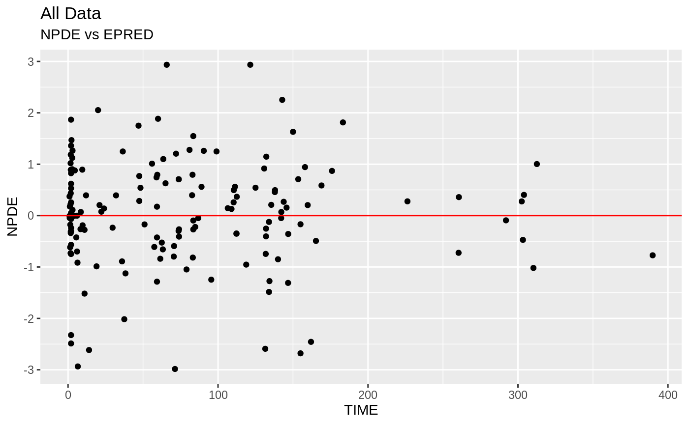
#> #   A1 <dbl>, EPRED <dbl>, ERES <dbl>, NPDE <dbl>

Basic Goodness of Fit Plots

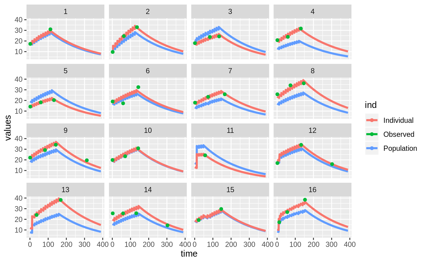
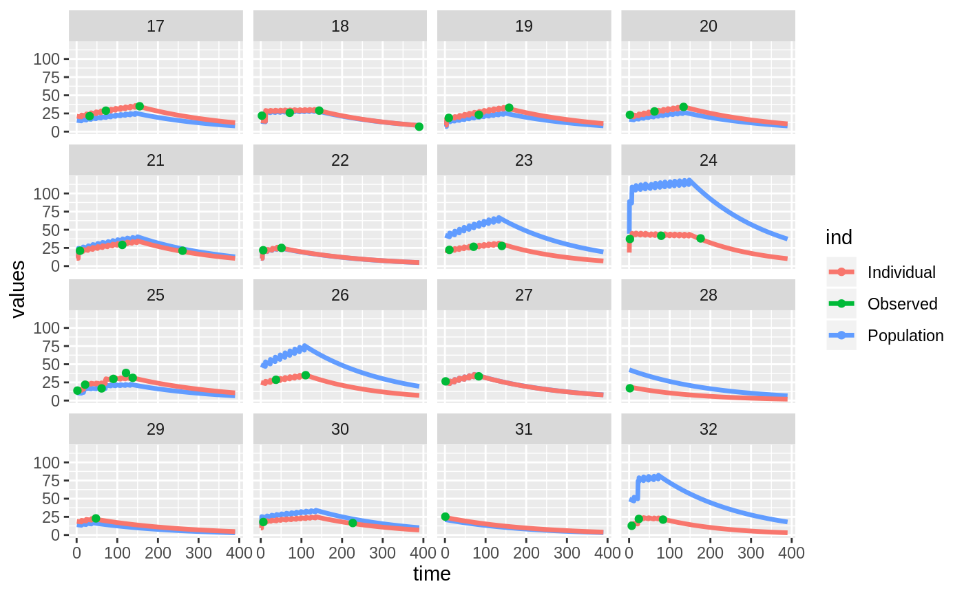
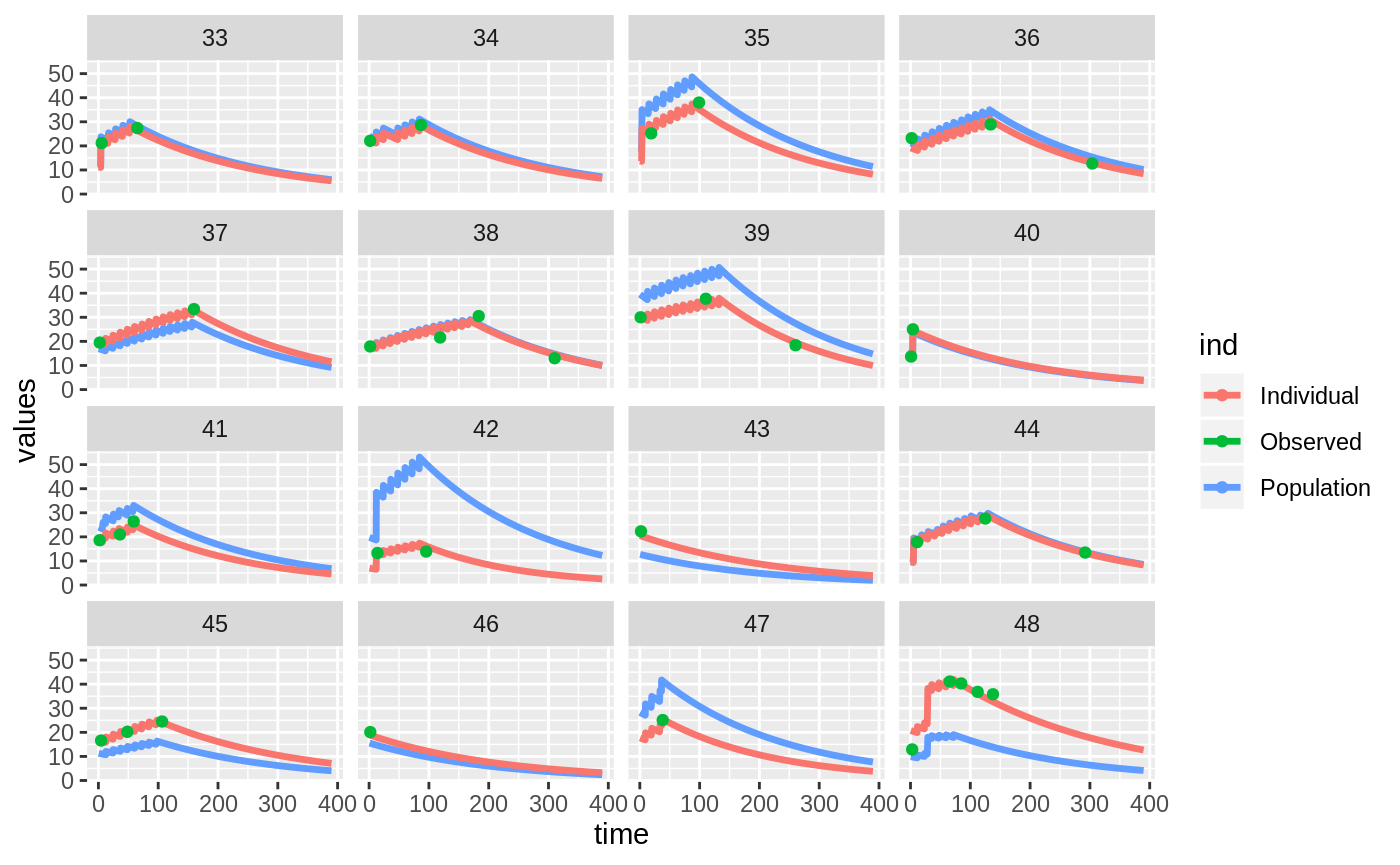
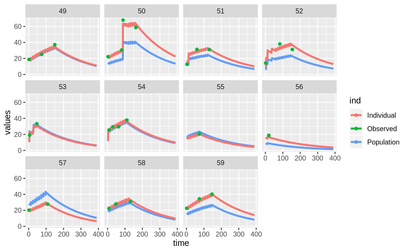
plot(fit)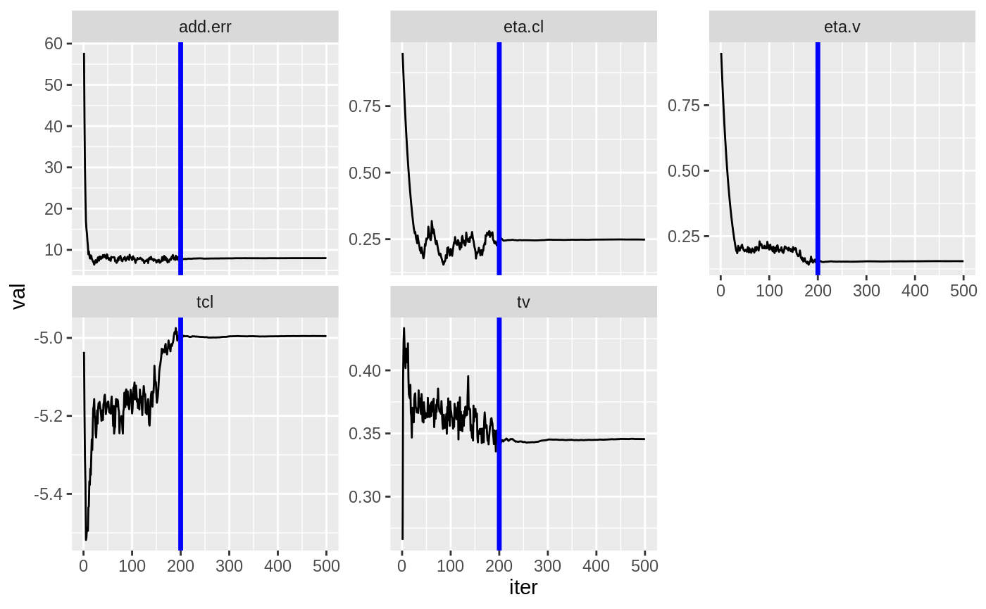

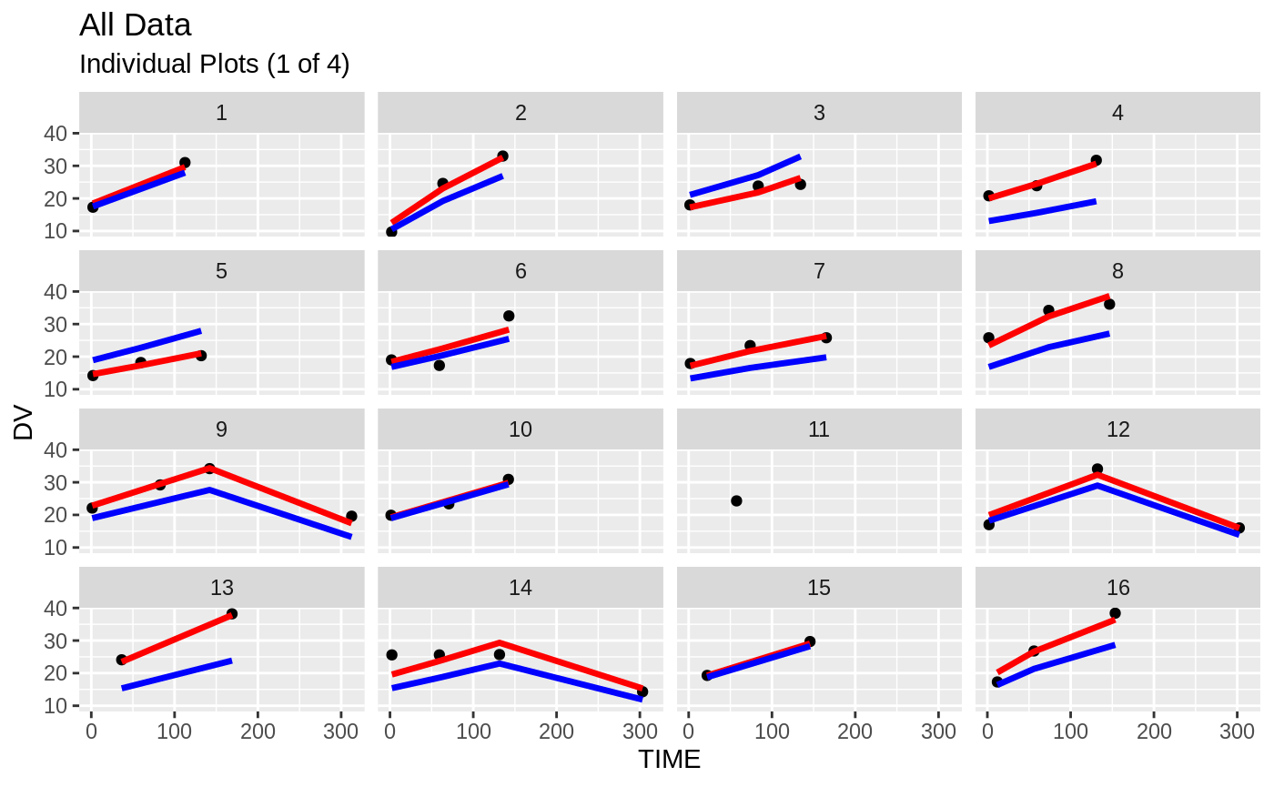
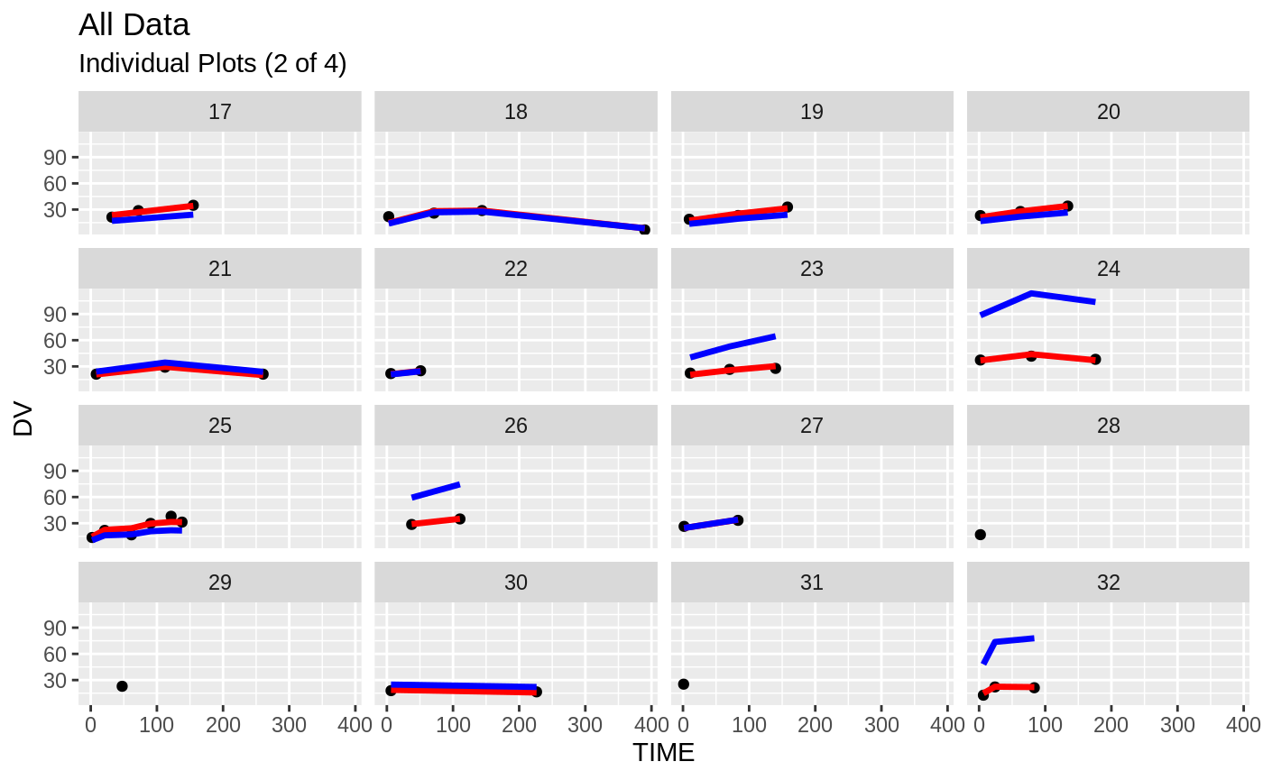
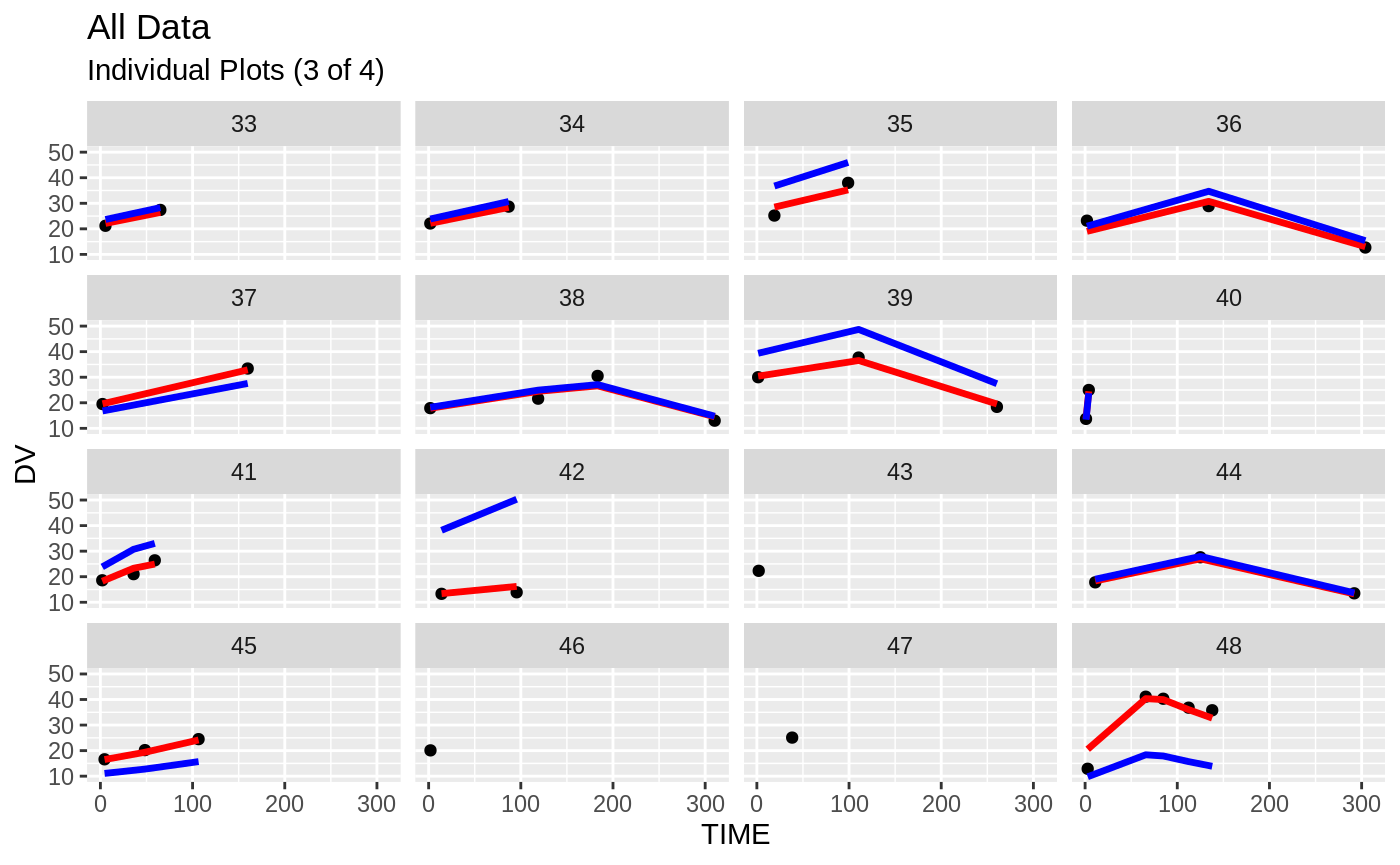
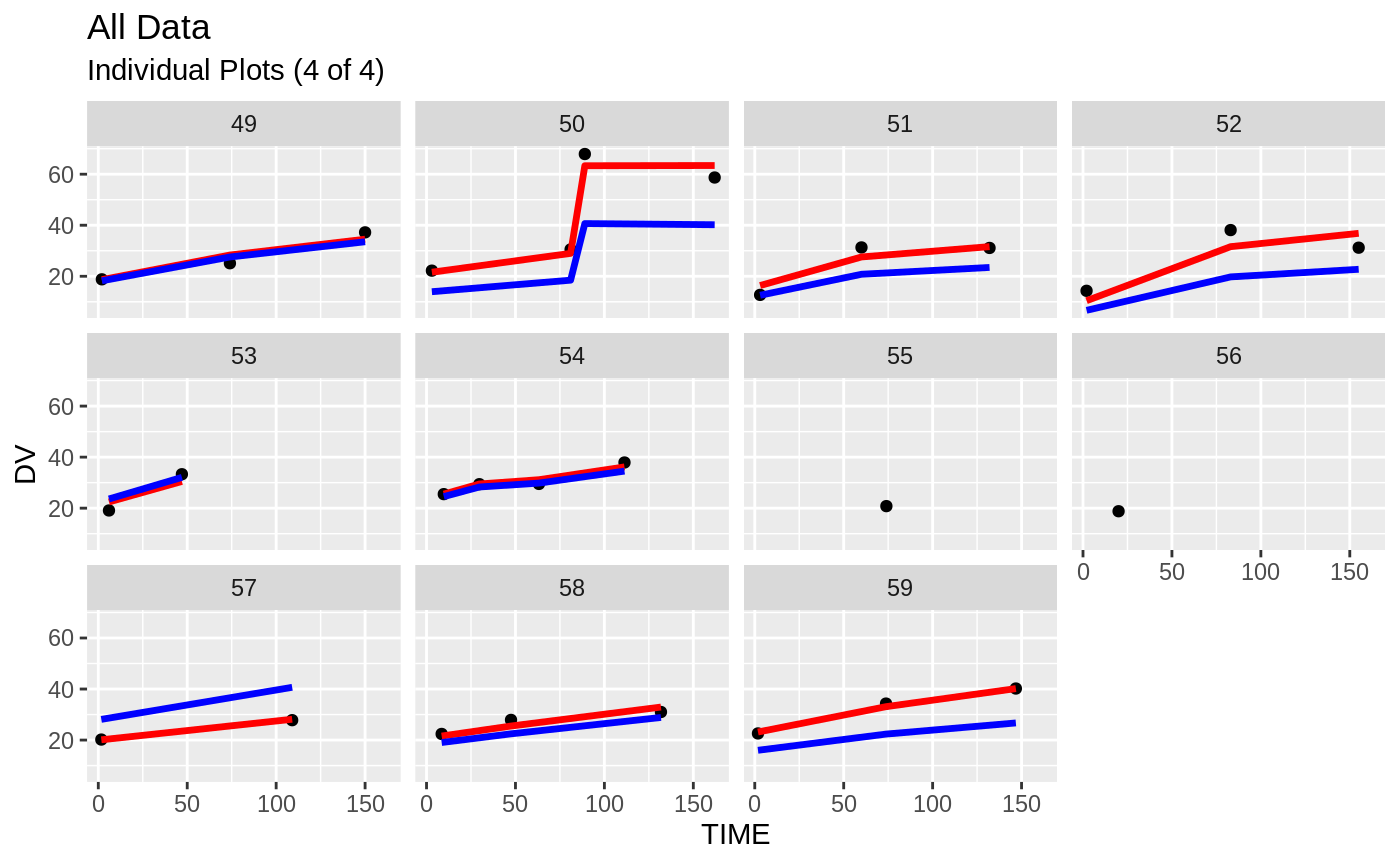
Those individual plots are not that great, it would be better to see the actual curves; You can with augPred

plot(augPred(fit))

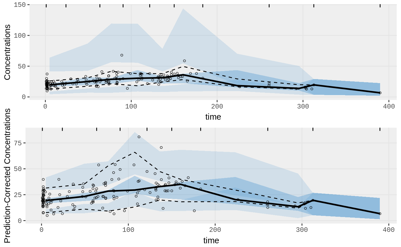
Two types of VPCs

library(ggplot2)
p1 <- nlmixr::vpc(fit, show=list(obs_dv=TRUE));
p1 <- p1+ ylab("Concentrations")

## A prediction-corrected VPC
p2 <- nlmixr::vpc(fit, pred_corr = TRUE, show=list(obs_dv=TRUE))
p2 <- p2+ ylab("Prediction-Corrected Concentrations")

library(gridExtra)
grid.arrange(p1,p2)