Chapter 12 Examples
This section is for example models to get you started in common simulation scenarios.
12.1 Prediction only models
Prediction only models are simple to create. You use the RxODE syntax without any ODE systems in them. A very simple example is a one-compartment model.
library(RxODE)
mod <- RxODE({
    ipre <- 10 * exp(-ke * t);
})
mod
#> RxODE 1.0.5 model named rx_7e31c1ae655db7c06244b075015b3e86 model (✔ ready).
#> x$params: ke
#> x$lhs: ipreSolving the RxODE models are the same as saving the simple ODE system, but faster of course.
et  <- et(seq(0,24,length.out=50))
cmt1 <- rxSolve(mod,et,params=c(ke=0.5))
cmt1
#> ▂▂▂▂▂▂▂▂▂▂▂▂▂▂▂▂▂▂▂▂ Solved RxODE object ▂▂▂▂▂▂▂▂▂▂▂▂▂▂▂▂▂▂▂
#> ── Parameters (x$params): ──────────────────────────────────
#> ke
#> 0.5
#> ── Initial Conditions (x$inits): ───────────────────────────
#> named numeric(0)
#> ── First part of data (object): ────────────────────────────
#> # A tibble: 50 x 2
#> time ipre
#> <dbl> <dbl>
#> 1 0 10
#> 2 0.490 7.83
#> 3 0.980 6.13
#> 4 1.47 4.80
#> 5 1.96 3.75
#> 6 2.45 2.94
#> # … with 44 more rows
#> ▂▂▂▂▂▂▂▂▂▂▂▂▂▂▂▂▂▂▂▂▂▂▂▂▂▂▂▂▂▂▂▂▂▂▂▂▂▂▂▂▂▂▂▂▂▂▂▂▂▂▂▂▂▂▂▂▂▂▂▂12.2 Solved compartment models
Solved models are also simple to create. You simply place the
linCmt() psuedo-function into your code. The linCmt() function
figures out the type of model to use based on the parameter names
specified.
Most often, pharmacometric models are parameterized in terms of volume
and clearances. Clearances are specified by NONMEM-style names of
CL, Q, Q1, Q2, etc. or distributional clearances CLD,
CLD2. Volumes are specified by Central (VC or V),
Peripheral/Tissue (VP, VT). While more translations are
available, some example translations are below:
Another popular parameterization is in terms of micro-constants. RxODE
assumes compartment 1 is the central compartment. The elimination
constant would be specified by K, Ke or Kel. Some example translations are below:
The last parameterization possible is using alpha and V and/or
A/B/C. Some example translations are below:
Once the linCmt() sleuthing is complete, the 1, 2 or 3
compartment model solution is used as the value of linCmt().
The compartments where you can dose in a linear solved system are
depot and central when there is an linear absorption constant in
the model ka. Without any additional ODEs, these compartments are
numbered depot=1 and central=2.
When the absorption constant ka is missing, you may only dose to the
central compartment. Without any additional ODEs the compartment
number is central=1.
These compartments take the same sort of events that a ODE model can take, and are discussed in the RxODE events vignette.
mod <- RxODE({
    ke <- 0.5
    V <- 1
    ipre <- linCmt();
})
mod
#> RxODE 1.0.5 model named rx_d41c572184c0c5d136339f94b81154e8 model (✔ ready).
#> x$stateExtra: central
#> x$params: ke, V
#> x$lhs: ipreThis then acts as an ODE model; You specify a dose to the depot compartment and then solve the system:
et  <- et(amt=10,time=0,cmt=depot) %>%
    et(seq(0,24,length.out=50))
cmt1 <- rxSolve(mod,et,params=c(ke=0.5))
cmt1
#> ▂▂▂▂▂▂▂▂▂▂▂▂▂▂▂▂▂▂▂▂ Solved RxODE object ▂▂▂▂▂▂▂▂▂▂▂▂▂▂▂▂▂▂▂
#> ── Parameters (x$params): ──────────────────────────────────
#> ke V
#> 0.5 1.0
#> ── Initial Conditions (x$inits): ───────────────────────────
#> named numeric(0)
#> ── First part of data (object): ────────────────────────────
#> # A tibble: 50 x 2
#> time ipre
#> <dbl> <dbl>
#> 1 0 10
#> 2 0.490 7.83
#> 3 0.980 6.13
#> 4 1.47 4.80
#> 5 1.96 3.75
#> 6 2.45 2.94
#> # … with 44 more rows
#> ▂▂▂▂▂▂▂▂▂▂▂▂▂▂▂▂▂▂▂▂▂▂▂▂▂▂▂▂▂▂▂▂▂▂▂▂▂▂▂▂▂▂▂▂▂▂▂▂▂▂▂▂▂▂▂▂▂▂▂▂12.3 Mixing Solved Systems and ODEs
In addition to pure ODEs, you may mix solved systems and ODEs. The
prior 2-compartment indirect response model can be simplified with a
linCmt() function:
library(RxODE)
## Setup example model
mod1 <-RxODE({
    C2 = centr/V2;
    C3 = peri/V3;
    d/dt(depot) =-KA*depot;
    d/dt(centr) = KA*depot - CL*C2 - Q*C2 + Q*C3;
    d/dt(peri)  =                    Q*C2 - Q*C3;
    d/dt(eff)  = Kin - Kout*(1-C2/(EC50+C2))*eff;
});

## Seup parameters and initial conditions

theta <-
    c(KA=2.94E-01, CL=1.86E+01, V2=4.02E+01, # central
      Q=1.05E+01,  V3=2.97E+02,              # peripheral
      Kin=1, Kout=1, EC50=200)               # effects

inits <- c(eff=1);

## Setup dosing event information
ev <- eventTable(amount.units="mg", time.units="hours") %>%
    add.dosing(dose=10000, nbr.doses=10, dosing.interval=12) %>%
    add.dosing(dose=20000, nbr.doses=5, start.time=120,dosing.interval=24) %>%
    add.sampling(0:240);

## Setup a mixed solved/ode system:
mod2 <- RxODE({
    ## the order of variables do not matter, the type of compartmental
    ## model is determined by the parameters specified.
    C2   = linCmt(KA, CL, V2, Q, V3);
    eff(0) = 1  ## This specifies that the effect compartment starts at 1.
    d/dt(eff) =  Kin - Kout*(1-C2/(EC50+C2))*eff;
})
This allows the indirect response model above to assign the
2-compartment model to the C2 variable and the used in the indirect
response model.
When mixing the solved systems and the ODEs, the solved system’s compartment is always the last compartment. This is because the solved system technically isn’t a compartment to be solved. Adding the dosing compartment to the end will not interfere with the actual ODE to be solved.
Therefore,in the two-compartment indirect response model, the effect compartment is compartment #1 while the PK dosing compartment for the depot is compartment #2.
This compartment model requires a new event table since the compartment number changed:
ev <- eventTable(amount.units='mg', time.units='hours') %>%
    add.dosing(dose=10000, nbr.doses=10, dosing.interval=12,dosing.to=2) %>%
    add.dosing(dose=20000, nbr.doses=5, start.time=120,dosing.interval=24,dosing.to=2) %>%
    add.sampling(0:240);
This can be solved with the following command:
x <- mod2 %>%  solve(theta, ev)
print(x)
#> ▂▂▂▂▂▂▂▂▂▂▂▂▂▂▂▂▂▂▂▂ Solved RxODE object ▂▂▂▂▂▂▂▂▂▂▂▂▂▂▂▂▂▂▂
#> ── Parameters ($params): ───────────────────────────────────
#> CL V2 Q V3 KA Kin Kout EC50
#> 18.600 40.200 10.500 297.000 0.294 1.000 1.000 200.000
#> ── Initial Conditions ($inits): ────────────────────────────
#> eff
#> 1
#> ── First part of data (object): ────────────────────────────
#> # A tibble: 241 x 3
#> time C2 eff
#> [h] <dbl> <dbl>
#> 1 0 249. 1
#> 2 1 121. 1.35
#> 3 2 60.3 1.38
#> 4 3 31.0 1.28
#> 5 4 17.0 1.18
#> 6 5 10.2 1.11
#> # … with 235 more rows
#> ▂▂▂▂▂▂▂▂▂▂▂▂▂▂▂▂▂▂▂▂▂▂▂▂▂▂▂▂▂▂▂▂▂▂▂▂▂▂▂▂▂▂▂▂▂▂▂▂▂▂▂▂▂▂▂▂▂▂▂▂Note this solving did not require specifying the effect compartment
initial condition to be 1. Rather, this is already pre-specified by eff(0)=1.
This can be solved for different initial conditions easily:
x <- mod2 %>%  solve(theta, ev,c(eff=2))
print(x)
#> ▂▂▂▂▂▂▂▂▂▂▂▂▂▂▂▂▂▂▂▂ Solved RxODE object ▂▂▂▂▂▂▂▂▂▂▂▂▂▂▂▂▂▂▂
#> ── Parameters ($params): ───────────────────────────────────
#> CL V2 Q V3 KA Kin Kout EC50
#> 18.600 40.200 10.500 297.000 0.294 1.000 1.000 200.000
#> ── Initial Conditions ($inits): ────────────────────────────
#> eff
#> 2
#> ── First part of data (object): ────────────────────────────
#> # A tibble: 241 x 3
#> time C2 eff
#> [h] <dbl> <dbl>
#> 1 0 249. 2
#> 2 1 121. 1.93
#> 3 2 60.3 1.67
#> 4 3 31.0 1.41
#> 5 4 17.0 1.23
#> 6 5 10.2 1.13
#> # … with 235 more rows
#> ▂▂▂▂▂▂▂▂▂▂▂▂▂▂▂▂▂▂▂▂▂▂▂▂▂▂▂▂▂▂▂▂▂▂▂▂▂▂▂▂▂▂▂▂▂▂▂▂▂▂▂▂▂▂▂▂▂▂▂▂The RxODE detective also does not require you to specify the variables
in the linCmt() function if they are already defined in the block.
Therefore, the following function will also work to solve the same
system.
mod3 <- RxODE({
    KA=2.94E-01;
    CL=1.86E+01;
    V2=4.02E+01;
    Q=1.05E+01;
    V3=2.97E+02;
    Kin=1;
    Kout=1;
    EC50=200;
    ## The linCmt() picks up the variables from above
    C2   = linCmt();
    eff(0) = 1  ## This specifies that the effect compartment starts at 1.
    d/dt(eff) =  Kin - Kout*(1-C2/(EC50+C2))*eff;
})

x <- mod3 %>%  solve(ev)
print(x)
#> ▂▂▂▂▂▂▂▂▂▂▂▂▂▂▂▂▂▂▂▂ Solved RxODE object ▂▂▂▂▂▂▂▂▂▂▂▂▂▂▂▂▂▂▂
#> ── Parameters ($params): ───────────────────────────────────
#> KA CL V2 Q V3 Kin Kout EC50
#> 0.294 18.600 40.200 10.500 297.000 1.000 1.000 200.000
#> ── Initial Conditions ($inits): ────────────────────────────
#> eff
#> 1
#> ── First part of data (object): ────────────────────────────
#> # A tibble: 241 x 3
#> time C2 eff
#> [h] <dbl> <dbl>
#> 1 0 249. 1
#> 2 1 121. 1.35
#> 3 2 60.3 1.38
#> 4 3 31.0 1.28
#> 5 4 17.0 1.18
#> 6 5 10.2 1.11
#> # … with 235 more rows
#> ▂▂▂▂▂▂▂▂▂▂▂▂▂▂▂▂▂▂▂▂▂▂▂▂▂▂▂▂▂▂▂▂▂▂▂▂▂▂▂▂▂▂▂▂▂▂▂▂▂▂▂▂▂▂▂▂▂▂▂▂Note that you do not specify the parameters when solving the system since they are built into the model, but you can override the parameters:
x <- mod3 %>%  solve(c(KA=10),ev)
print(x)
#> ▂▂▂▂▂▂▂▂▂▂▂▂▂▂▂▂▂▂▂▂ Solved RxODE object ▂▂▂▂▂▂▂▂▂▂▂▂▂▂▂▂▂▂▂
#> ── Parameters ($params): ───────────────────────────────────
#> KA CL V2 Q V3 Kin Kout EC50
#> 10.0 18.6 40.2 10.5 297.0 1.0 1.0 200.0
#> ── Initial Conditions ($inits): ────────────────────────────
#> eff
#> 1
#> ── First part of data (object): ────────────────────────────
#> # A tibble: 241 x 3
#> time C2 eff
#> [h] <dbl> <dbl>
#> 1 0 249. 1
#> 2 1 121. 1.35
#> 3 2 60.3 1.38
#> 4 3 31.0 1.28
#> 5 4 17.0 1.18
#> 6 5 10.2 1.11
#> # … with 235 more rows
#> ▂▂▂▂▂▂▂▂▂▂▂▂▂▂▂▂▂▂▂▂▂▂▂▂▂▂▂▂▂▂▂▂▂▂▂▂▂▂▂▂▂▂▂▂▂▂▂▂▂▂▂▂▂▂▂▂▂▂▂▂12.4 Weight based dosing
This is an example model for weight based dosing of daptomycin. Daptomycin is a cyclic lipopeptide antibiotic from fermented Streptomyces roseosporus.
There are 3 stages for weight-based dosing simulations: - Create RxODE model - Simulate Covariates - Create event table with weight-based dosing (merged back to covariates)
12.4.1 Creating a 2-compartment model in RxODE
library(RxODE)

## Note the time covariate is not included in the simulation
m1 <- RxODE({
  CL ~ (1-0.2*SEX)*(0.807+0.00514*(CRCL-91.2))*exp(eta.cl)
  V1 ~ 4.8*exp(eta.v1)
  Q ~ (3.46+0.0593*(WT-75.1))*exp(eta.q);
  V2 ~ 1.93*(3.13+0.0458*(WT-75.1))*exp(eta.v2)
  A1 ~ centr;
  A2 ~ peri;
  d/dt(centr) ~ - A1*(CL/V1 + Q/V1) + A2*Q/V2;
  d/dt(peri) ~ A1*Q/V1 - A2*Q/V2;
  DV = centr / V1 * (1 + prop.err)
})
12.4.2 Simulating Covariates
This simulation correlates age, sex, and weight. Since we will be using weight based dosing, this needs to be simulated first
set.seed(42)
library(dplyr)
nsub=30
### Simulate Weight based on age and gender
AGE<-round(runif(nsub,min=18,max=70))
SEX<-round(runif(nsub,min=0,max=1))
HTm<-round(rnorm(nsub,176.3,0.17*sqrt(4482)),digits=1)
HTf<-round(rnorm(nsub,162.2,0.16*sqrt(4857)),digits=1)
WTm<-round(exp(3.28+1.92*log(HTm/100))*exp(rnorm(nsub,0,0.14)),digits=1)
WTf<-round(exp(3.49+1.45*log(HTf/100))*exp(rnorm(nsub,0,0.17)),digits=1)
WT<-ifelse(SEX==1,WTf,WTm)
CRCL<-round(runif(nsub,30,140))
## id is in lower case to match the event table
cov.df <- tibble(id=seq_along(AGE), AGE=AGE, SEX=SEX, WT=WT, CRCL=CRCL)
print(cov.df)
#> # A tibble: 30 x 5
#> id AGE SEX WT CRCL
#> <int> <dbl> <dbl> <dbl> <dbl>
#> 1 1 66 1 49.4 83
#> 2 2 67 1 52.5 79
#> 3 3 33 0 97.9 37
#> 4 4 61 1 63.8 66
#> 5 5 51 0 71.8 127
#> 6 6 45 1 69.6 132
#> 7 7 56 0 61 73
#> 8 8 25 0 57.7 47
#> 9 9 52 1 58.7 65
#> 10 10 55 1 73.1 64
#> # ... with 20 more rows12.4.3 Creating weight based event table
s<-c(0,0.25,0.5,0.75,1,1.5,seq(2,24,by=1))
s <- lapply(s, function(x){.x <- 0.1 * x; c(x - .x, x + .x)})

e <- et() %>%
    ## Specify the id and weight based dosing from covariate data.frame
    ## This requires RxODE XXX
    et(id=cov.df$id, amt=6*cov.df$WT, rate=6 * cov.df$WT) %>%
    ## Sampling is added for each ID
    et(s) %>%
    as.data.frame %>%
    ## Merge the event table with the covarite information
    merge(cov.df, by="id") %>%
    as_tibble


e
#> # A tibble: 900 x 12
#> id low time high cmt amt rate evid AGE SEX WT CRCL
#> <int> <dbl> <dbl> <dbl> <chr> <dbl> <dbl> <int> <dbl> <dbl> <dbl> <dbl>
#> 1 1 0 0 0 (obs) NA NA 0 66 1 49.4 83
#> 2 1 NA 0 NA (default) 296. 296. 1 66 1 49.4 83
#> 3 1 0.225 0.246 0.275 (obs) NA NA 0 66 1 49.4 83
#> 4 1 0.45 0.516 0.55 (obs) NA NA 0 66 1 49.4 83
#> 5 1 0.675 0.729 0.825 (obs) NA NA 0 66 1 49.4 83
#> 6 1 0.9 0.921 1.1 (obs) NA NA 0 66 1 49.4 83
#> 7 1 1.35 1.42 1.65 (obs) NA NA 0 66 1 49.4 83
#> 8 1 1.8 1.82 2.2 (obs) NA NA 0 66 1 49.4 83
#> 9 1 2.7 2.97 3.3 (obs) NA NA 0 66 1 49.4 83
#> 10 1 3.6 3.87 4.4 (obs) NA NA 0 66 1 49.4 83
#> # ... with 890 more rows12.4.4 Solving Daptomycin simulation
data <- rxSolve(m1, e,
             ## Lotri uses lower-triangular matrix rep. for named matrix
             omega=lotri(eta.cl ~ .306,
                         eta.q ~0.0652,
                         eta.v1 ~.567,
                         eta.v2 ~ .191),
             sigma=lotri(prop.err ~ 0.15),
             addDosing = TRUE, addCov = TRUE)

print(data)
#> ______________________________ Solved RxODE object _____________________________
#> -- Parameters ($params): -------------------------------------------------------
#> # A tibble: 30 x 5
#> id eta.cl eta.v1 eta.q eta.v2
#> <fct> <dbl> <dbl> <dbl> <dbl>
#> 1 1 0.563 0.580 0.0360 -0.246
#> 2 2 0.0341 0.406 -0.139 -0.481
#> 3 3 -0.447 0.0952 -0.185 -0.249
#> 4 4 -0.988 0.248 -0.131 -0.449
#> 5 5 0.144 -1.14 0.106 0.360
#> 6 6 -0.689 0.407 -0.193 -0.200
#> 7 7 -0.426 -0.706 -0.190 -0.234
#> 8 8 -0.212 0.728 0.335 0.0665
#> 9 9 0.0884 -0.934 0.337 0.154
#> 10 10 -0.557 1.29 0.0163 -0.140
#> # ... with 20 more rows
#> -- Initial Conditions ($inits): ------------------------------------------------
#> centr peri
#> 0 0
#> -- First part of data (object): ------------------------------------------------
#> # A tibble: 900 x 9
#> id evid cmt amt time DV SEX WT CRCL
#> <int> <int> <int> <dbl> <dbl> <dbl> <dbl> <dbl> <dbl>
#> 1 1 1 1 296. 0 0 1 49.4 83
#> 2 1 0 NA NA 0 0 1 49.4 83
#> 3 1 0 NA NA 0.246 2.32 1 49.4 83
#> 4 1 0 NA NA 0.516 19.6 1 49.4 83
#> 5 1 0 NA NA 0.729 23.2 1 49.4 83
#> 6 1 0 NA NA 0.921 21.1 1 49.4 83
#> # ... with 894 more rows
#> ________________________________________________________________________________plot(data, log="y")#> Warning in self$trans$transform(x): NaNs produced#> Warning: Transformation introduced infinite values in continuous y-axis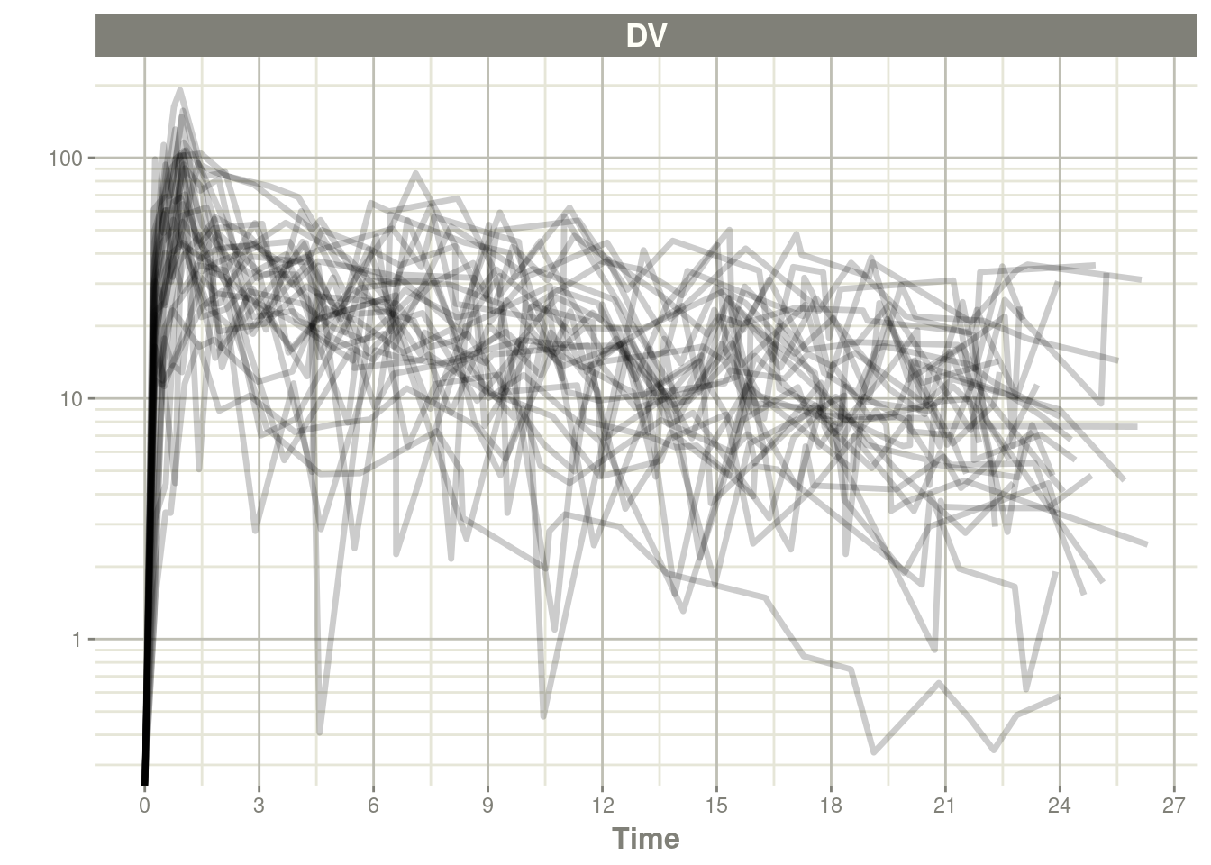
12.4.5 Daptomycin Reference
This weight-based simulation is adapted from the Daptomycin article below:
Dvorchik B, Arbeit RD, Chung J, Liu S, Knebel W, Kastrissios H. Population pharmacokinetics of daptomycin. Antimicrob Agents Che mother 2004; 48: 2799-2807. doi:(10.1128/AAC.48.8.2799-2807.2004)[https://dx.doi.org/10.1128%2FAAC.48.8.2799-2807.2004]
This simulation example was made available from the work of Sherwin Sy with modifications by Matthew Fidler
12.5 Inter-occasion and other nesting examples
More than one level of nesting is possible in RxODE; In this example we will be using the following uncertainties and sources of variability:
| Level | Variable | Matrix specified | Integrated Matrix |
|---|---|---|---|
| Model uncertainty | NA | thetaMat |
thetaMat |
| Investigator | inv.Cl, inv.Ka |
omega |
theta |
| Subject | eta.Cl, eta.Ka |
omega |
omega |
| Eye | eye.Cl, eye.Ka |
omega |
omega |
| Occasion | iov.Cl, occ.Ka |
omega |
omega |
| Unexplained Concentration | prop.sd |
sigma |
sigma |
| Unexplained Effect | add.sd |
sigma |
sigma |
12.5.1 Event table
This event table contains nesting variables:
- inv: investigator id
- id: subject id
- eye: eye id (left or right)
- occ: occasion
library(RxODE)
library(dplyr)

et(amountUnits="mg", timeUnits="hours") %>%
  et(amt=10000, addl=9,ii=12,cmt="depot") %>%
  et(time=120, amt=2000, addl=4, ii=14, cmt="depot") %>%
  et(seq(0, 240, by=4)) %>% # Assumes sampling when there is no dosing information
  et(seq(0, 240, by=4) + 0.1) %>% ## adds 0.1 for separate eye
  et(id=1:20) %>%
  ## Add an occasion per dose
  mutate(occ=cumsum(!is.na(amt))) %>%
  mutate(occ=ifelse(occ == 0, 1, occ)) %>%
  mutate(occ=2- occ %% 2) %>%
  mutate(eye=ifelse(round(time) == time, 1, 2)) %>%
  mutate(inv=ifelse(id < 10, 1, 2)) %>% as_tibble ->
  ev
12.5.2 RxODE model
This creates the RxODE model with multi-level nesting. Note the
variables inv.Cl, inv.Ka, eta.Cl etc; You only need one variable
for each level of nesting.
mod <- RxODE({
  ## Clearance with individuals
  eff(0) = 1
  C2 = centr/V2*(1+prop.sd);
  C3 = peri/V3;
  CL =  TCl*exp(eta.Cl + eye.Cl + iov.Cl + inv.Cl)
  KA = TKA * exp(eta.Ka + eye.Ka + iov.Cl + inv.Ka)
  d/dt(depot) =-KA*depot;
  d/dt(centr) = KA*depot - CL*C2 - Q*C2 + Q*C3;
  d/dt(peri)  =                    Q*C2 - Q*C3;
  d/dt(eff)  = Kin - Kout*(1-C2/(EC50+C2))*eff;
  ef0 = eff + add.sd
})
12.5.3 Uncertainty in Model parameters
theta <- c("TKA"=0.294, "TCl"=18.6, "V2"=40.2,
           "Q"=10.5, "V3"=297, "Kin"=1, "Kout"=1, "EC50"=200)

## Creating covariance matrix
tmp <- matrix(rnorm(8^2), 8, 8)
tMat <- tcrossprod(tmp, tmp) / (8 ^ 2)
dimnames(tMat) <- list(names(theta), names(theta))

tMat
#> TKA TCl V2 Q V3
#> TKA 0.084901793 0.008491535 -0.028211905 -0.083460075 0.058187918
#> TCl 0.008491535 0.074011602 -0.047388281 -0.049711532 0.009450000
#> V2 -0.028211905 -0.047388281 0.094485793 -0.001142105 -0.031424916
#> Q -0.083460075 -0.049711532 -0.001142105 0.271685090 -0.042012559
#> V3 0.058187918 0.009450000 -0.031424916 -0.042012559 0.089992792
#> Kin -0.046169545 -0.016205743 -0.014705754 0.094478654 0.001534101
#> Kout -0.023946567 -0.040201822 0.008377087 0.062087105 -0.053276590
#> EC50 -0.017733886 -0.011145761 -0.004038295 0.025496213 0.006360558
#> Kin Kout EC50
#> TKA -0.046169545 -0.023946567 -0.017733886
#> TCl -0.016205743 -0.040201822 -0.011145761
#> V2 -0.014705754 0.008377087 -0.004038295
#> Q 0.094478654 0.062087105 0.025496213
#> V3 0.001534101 -0.053276590 0.006360558
#> Kin 0.102223150 0.035112776 0.030704006
#> Kout 0.035112776 0.109746574 0.019060142
#> EC50 0.030704006 0.019060142 0.03018868812.5.4 Nesting Variability
To specify multiple levels of nesting, you can specify it as a nested
lotri matrix; When using this approach you use the condition
operator | to specify what variable nesting occurs on; For the
Bayesian simulation we need to specify how much information we have
for each parameter; For RxODE this is the nu parameter.
In this case:
- id, nu=100 or the model came from 100 subjects
- eye, nu=200 or the model came from 200 eyes
- occ, nu=200 or the model came from 200 occasions
- inv, nu=10 or the model came from 10 investigators
To specify this in lotri you can use | var(nu=X), or:
omega <- lotri(lotri(eta.Cl ~ 0.1,
                     eta.Ka ~ 0.1) | id(nu=100),
               lotri(eye.Cl ~ 0.05,
                     eye.Ka ~ 0.05) | eye(nu=200),
               lotri(iov.Cl ~ 0.01,
                     iov.Ka ~ 0.01) | occ(nu=200),
               lotri(inv.Cl ~ 0.02,
                     inv.Ka ~ 0.02) | inv(nu=10))
omega
#> $id
#> eta.Cl eta.Ka
#> eta.Cl 0.1 0.0
#> eta.Ka 0.0 0.1
#>
#> $eye
#> eye.Cl eye.Ka
#> eye.Cl 0.05 0.00
#> eye.Ka 0.00 0.05
#>
#> $occ
#> iov.Cl iov.Ka
#> iov.Cl 0.01 0.00
#> iov.Ka 0.00 0.01
#>
#> $inv
#> inv.Cl inv.Ka
#> inv.Cl 0.02 0.00
#> inv.Ka 0.00 0.02
#>
#> Properties: nu12.5.5 Unexplained variability
The last piece of variability to specify is the unexplained variability
sigma <- lotri(prop.sd ~ .25,
               add.sd~ 0.125)
12.5.6 Solving the problem
s <- rxSolve(mod, theta, ev,
             thetaMat=tMat, omega=omega,
             sigma=sigma, sigmaDf=400,
             nStud=400)
#> unhandled error message: EE:[lsoda] 70000 steps taken before reaching tout
#> @(lsoda.c:748#> Warning: some ID(s) could not solve the ODEs correctly; These values are
#> replaced with 'NA'print(s)#> ______________________________ Solved RxODE object _____________________________
#> -- Parameters ($params): -------------------------------------------------------
#> # A tibble: 8,000 x 24
#> sim.id id `inv.Cl(inv==1)` `inv.Cl(inv==2)` `inv.Ka(inv==1)`
#> <int> <fct> <dbl> <dbl> <dbl>
#> 1 1 1 0.0186 0.116 0.188
#> 2 1 2 0.0186 0.116 0.188
#> 3 1 3 0.0186 0.116 0.188
#> 4 1 4 0.0186 0.116 0.188
#> 5 1 5 0.0186 0.116 0.188
#> 6 1 6 0.0186 0.116 0.188
#> 7 1 7 0.0186 0.116 0.188
#> 8 1 8 0.0186 0.116 0.188
#> 9 1 9 0.0186 0.116 0.188
#> 10 1 10 0.0186 0.116 0.188
#> # ... with 7,990 more rows, and 19 more variables: inv.Ka(inv==2) <dbl>,
#> # eye.Cl(eye==1) <dbl>, eye.Cl(eye==2) <dbl>, eye.Ka(eye==1) <dbl>,
#> # eye.Ka(eye==2) <dbl>, iov.Cl(occ==1) <dbl>, iov.Cl(occ==2) <dbl>,
#> # iov.Ka(occ==1) <dbl>, iov.Ka(occ==2) <dbl>, V2 <dbl>, V3 <dbl>, TCl <dbl>,
#> # eta.Cl <dbl>, TKA <dbl>, eta.Ka <dbl>, Q <dbl>, Kin <dbl>, Kout <dbl>,
#> # EC50 <dbl>
#> -- Initial Conditions ($inits): ------------------------------------------------
#> depot centr peri eff
#> 0 0 0 1
#>
#> Simulation with uncertainty in:
#> * parameters (s$thetaMat for changes)
#> * omega matrix (s$omegaList)
#>
#> -- First part of data (object): ------------------------------------------------
#> # A tibble: 976,000 x 18
#> sim.id id time inv.Cl inv.Ka eye.Cl eye.Ka iov.Cl iov.Ka C2 C3
#> <int> <int> [h] <dbl> <dbl> <dbl> <dbl> <dbl> <dbl> <dbl> <dbl>
#> 1 1 1 0.0 0.0186 0.188 -0.104 0.0786 0.0247 -0.0530 0 0
#> 2 1 1 0.1 0.0186 0.188 -0.296 0.0588 0.0247 -0.0530 3.00 0.0281
#> 3 1 1 4.0 0.0186 0.188 -0.104 0.0786 0.0247 -0.0530 22.4 9.90
#> 4 1 1 4.1 0.0186 0.188 -0.296 0.0588 0.0247 -0.0530 57.9 10.1
#> 5 1 1 8.0 0.0186 0.188 -0.104 0.0786 0.0247 -0.0530 20.1 12.4
#> 6 1 1 8.1 0.0186 0.188 -0.296 0.0588 0.0247 -0.0530 15.6 12.4
#> # ... with 975,994 more rows, and 7 more variables: CL <dbl>, KA <dbl>,
#> # ef0 <dbl>, depot <dbl>, centr <dbl>, peri <dbl>, eff <dbl>
#> ________________________________________________________________________________There are multiple investigators in a study; Each investigator has a
number of individuals enrolled at their site. RxODE automatically
determines the number of investigators and then will simulate an
effect for each investigator. With the output, inv.Cl(inv==1) will
be the inv.Cl for investigator 1, inv.Cl(inv==2) will be the
inv.Cl for investigator 2, etc.
inv.Cl(inv==1), inv.Cl(inv==2), etc will be simulated for each
study and then combined to form the between investigator
variability. In equation form these represent the following:
inv.Cl = (inv == 1) * `inv.Cl(inv==1)` + (inv == 2) * `inv.Cl(inv==2)`If you look at the simulated parameters you can see inv.Cl(inv==1)
and inv.Cl(inv==2) are in the s$params; They are the same for each
study:
print(head(s$params))#> sim.id id inv.Cl(inv==1) inv.Cl(inv==2) inv.Ka(inv==1) inv.Ka(inv==2)
#> 1 1 1 0.01864161 0.1159198 0.1878234 -0.292727
#> 2 1 2 0.01864161 0.1159198 0.1878234 -0.292727
#> 3 1 3 0.01864161 0.1159198 0.1878234 -0.292727
#> 4 1 4 0.01864161 0.1159198 0.1878234 -0.292727
#> 5 1 5 0.01864161 0.1159198 0.1878234 -0.292727
#> 6 1 6 0.01864161 0.1159198 0.1878234 -0.292727
#> eye.Cl(eye==1) eye.Cl(eye==2) eye.Ka(eye==1) eye.Ka(eye==2) iov.Cl(occ==1)
#> 1 -0.10410790 -0.29632211 0.07855205 0.05884539 0.02466606
#> 2 -0.06820792 0.06585538 0.34603340 0.20141355 -0.06976537
#> 3 -0.04885836 0.13135196 -0.13256387 0.21645151 -0.03121109
#> 4 0.20667975 -0.08775327 -0.01404241 -0.04239568 -0.08207797
#> 5 0.04877033 -0.22890756 -0.21685969 0.04846680 -0.01393029
#> 6 0.19830134 -0.33204702 -0.16960164 0.06823678 -0.17462695
#> iov.Cl(occ==2) iov.Ka(occ==1) iov.Ka(occ==2) V2 V3 TCl
#> 1 -0.11264526 -0.052971164 -0.106088075 39.57653 297.3736 18.81115
#> 2 0.03970507 -0.073742566 0.090882718 39.57653 297.3736 18.81115
#> 3 -0.23892944 -0.136470596 0.067412442 39.57653 297.3736 18.81115
#> 4 -0.02134625 -0.061910605 -0.072601879 39.57653 297.3736 18.81115
#> 5 0.05580236 0.099876044 -0.094708943 39.57653 297.3736 18.81115
#> 6 -0.03152016 -0.002074008 -0.004758332 39.57653 297.3736 18.81115
#> eta.Cl TKA eta.Ka Q Kin Kout EC50
#> 1 -0.02740884 0.4375889 0.07529548 10.97588 1.179938 0.9161172 200.2625
#> 2 -0.11896272 0.4375889 0.07490355 10.97588 1.179938 0.9161172 200.2625
#> 3 -0.61026874 0.4375889 -0.15964154 10.97588 1.179938 0.9161172 200.2625
#> 4 -0.17447915 0.4375889 -0.19377239 10.97588 1.179938 0.9161172 200.2625
#> 5 0.26213020 0.4375889 -0.38954283 10.97588 1.179938 0.9161172 200.2625
#> 6 -0.22932331 0.4375889 -0.49123723 10.97588 1.179938 0.9161172 200.2625print(head(s$params %>% filter(sim.id == 2)))#> sim.id id inv.Cl(inv==1) inv.Cl(inv==2) inv.Ka(inv==1) inv.Ka(inv==2)
#> 1 2 1 -0.01105301 -0.1209402 0.3370577 0.0902204
#> 2 2 2 -0.01105301 -0.1209402 0.3370577 0.0902204
#> 3 2 3 -0.01105301 -0.1209402 0.3370577 0.0902204
#> 4 2 4 -0.01105301 -0.1209402 0.3370577 0.0902204
#> 5 2 5 -0.01105301 -0.1209402 0.3370577 0.0902204
#> 6 2 6 -0.01105301 -0.1209402 0.3370577 0.0902204
#> eye.Cl(eye==1) eye.Cl(eye==2) eye.Ka(eye==1) eye.Ka(eye==2) iov.Cl(occ==1)
#> 1 -0.01262553 -0.08161227 -0.238499594 0.17178813 0.08330981
#> 2 -0.06778157 0.29410669 -0.003700213 -0.03805489 -0.12869095
#> 3 0.06059738 -0.16831575 -0.085582067 0.22970053 0.05711749
#> 4 -0.13086494 0.02748735 -0.056454551 -0.23331112 0.07216869
#> 5 -0.23416424 -0.13568099 -0.436719663 -0.03106162 -0.13191139
#> 6 0.24092815 0.66166495 -0.345840539 0.13552870 0.03987511
#> iov.Cl(occ==2) iov.Ka(occ==1) iov.Ka(occ==2) V2 V3 TCl
#> 1 -0.148592318 0.10100830 0.050123275 40.32538 296.5826 18.65152
#> 2 -0.002200205 -0.04045931 -0.077835601 40.32538 296.5826 18.65152
#> 3 -0.185116411 0.02903611 0.076384740 40.32538 296.5826 18.65152
#> 4 0.101902663 0.04680555 0.054662894 40.32538 296.5826 18.65152
#> 5 0.103696663 0.02589958 0.100946619 40.32538 296.5826 18.65152
#> 6 0.023244426 -0.03067335 -0.009347601 40.32538 296.5826 18.65152
#> eta.Cl TKA eta.Ka Q Kin Kout EC50
#> 1 -0.2518665 -0.2160777 0.33092617 11.02462 1.122102 1.022177 199.9981
#> 2 0.3495104 -0.2160777 -0.35774607 11.02462 1.122102 1.022177 199.9981
#> 3 -0.3101379 -0.2160777 -0.09014428 11.02462 1.122102 1.022177 199.9981
#> 4 -0.1665144 -0.2160777 -0.11974060 11.02462 1.122102 1.022177 199.9981
#> 5 0.3184297 -0.2160777 -0.06982612 11.02462 1.122102 1.022177 199.9981
#> 6 -0.1216137 -0.2160777 0.30275205 11.02462 1.122102 1.022177 199.9981For between eye variability and between occasion variability each individual simulates a number of variables that become the between eye and between occasion variability; In the case of the eye:
eye.Cl = (eye == 1) * `eye.Cl(eye==1)` + (eye == 2) * `eye.Cl(eye==2)`So when you look the simulation each of these variables (ie
eye.Cl(eye==1), eye.Cl(eye==2), etc) they change for each
individual and when combined make the between eye variability or the
between occasion variability that can be seen in some pharamcometric
models.
12.6 Transit compartment models
Savic 2008 first introduced the idea of transit compartments being a mechanistic explanation of a a lag-time type phenomena. RxODE has special handling of these models:
You can specify this in a similar manner as the original paper:
library(RxODE)
mod <- RxODE({
    ## Table 3 from Savic 2007
    cl = 17.2 # (L/hr)
    vc = 45.1 # L
    ka = 0.38 # 1/hr
    mtt = 0.37 # hr
    bio=1
    n = 20.1
    k = cl/vc
    ktr = (n+1)/mtt
    ## note that lgammafn is the same as lgamma in R.
    d/dt(depot) = exp(log(bio*podo)+log(ktr)+n*log(ktr*t)-ktr*t-lgammafn(n+1))-ka*depot
    d/dt(cen) = ka*depot-k*cen
})

et <- eventTable();
et$add.sampling(seq(0, 7, length.out=200));
et$add.dosing(20, start.time=0);

transit <- rxSolve(mod, et, transit_abs=TRUE)

plot(transit, cen, ylab="Central Concentration")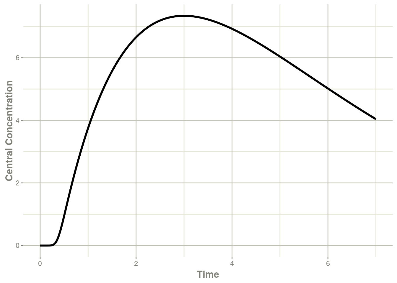
Another option is to specify the transit compartment function
transit syntax. This specifies the parameters transit(number of transit compartments, mean transit time, bioavailability). The
bioavailability term is optional.
Using the transit code also automatically turns on the transit_abs
option. Therefore, the same model can be specified by:
mod <- RxODE({
    ## Table 3 from Savic 2007
    cl = 17.2 # (L/hr)
    vc = 45.1 # L
    ka = 0.38 # 1/hr
    mtt = 0.37 # hr
    bio=1
    n = 20.1
    k = cl/vc
    ktr = (n+1)/mtt
    d/dt(depot) = transit(n,mtt,bio)-ka*depot
    d/dt(cen) = ka*depot-k*cen
})

et <- eventTable();
et$add.sampling(seq(0, 7, length.out=200));
et$add.dosing(20, start.time=0);

transit <- rxSolve(mod, et)
#> Warning: assumed transit compartment model since 'podo' is in the modelplot(transit, cen, ylab="Central Concentration")