Chapter 13 Advanced & Miscellaneous Topics

This covers advanced or miscellaneous topics in RxODE

13.1 Covariates in RxODE

13.1.1 Individual Covariates

If there is an individual covariate you wish to solve for you may specify it by the iCov dataset:

library(RxODE)
library(units)
library(xgxr)

mod3 <- RxODE({
    KA=2.94E-01;
#### Clearance with individuals
    CL=1.86E+01 * (WT / 70) ^ 0.75;
    V2=4.02E+01;
    Q=1.05E+01;
    V3=2.97E+02;
    Kin=1;
    Kout=1;
    EC50=200;
#### The linCmt() picks up the variables from above
    C2   = linCmt();
    Tz= 8
    amp=0.1
    eff(0) = 1  ## This specifies that the effect compartment starts at 1.
    d/dt(eff) =  Kin - Kout*(1-C2/(EC50+C2))*eff;
})

ev <- et(amount.units="mg", time.units="hours") %>%
    et(amt=10000, cmt=1) %>%
    et(0,48,length.out=100) %>%
    et(id=1:4);

set.seed(10)
#### Now use iCov to simulate a 4-id sample
r1 <- solve(mod3, ev,
### Create individual covariate data-frame
            iCov=data.frame(id=1:4, WT=rnorm(4, 70, 10)),
### in this case it would be useful to keep the WT in the output dataset
            keep="WT")
print(r1)

#> ______________________________ Solved RxODE object _____________________________
#> -- Parameters ($params): -------------------------------------------------------
#> # A tibble: 4 x 11
#>   id       KA    WT    V2     Q    V3   Kin  Kout  EC50    Tz   amp
#>   <fct> <dbl> <dbl> <dbl> <dbl> <dbl> <dbl> <dbl> <dbl> <dbl> <dbl>
#> 1 1     0.294  70.2  40.2  10.5   297     1     1   200     8   0.1
#> 2 2     0.294  68.2  40.2  10.5   297     1     1   200     8   0.1
#> 3 3     0.294  56.3  40.2  10.5   297     1     1   200     8   0.1
#> 4 4     0.294  64.0  40.2  10.5   297     1     1   200     8   0.1
#> -- Initial Conditions ($inits): ------------------------------------------------
#> eff 
#>   1 
#> -- First part of data (object): ------------------------------------------------
#> # A tibble: 400 x 6
#>      id      time    CL    C2   eff    WT
#>   <int>       [h] <dbl> <dbl> <dbl> <dbl>
#> 1     1 0.0000000  18.6   0    1     70.2
#> 2     1 0.4848485  18.6  27.8  1.03  70.2
#> 3     1 0.9696970  18.6  43.7  1.08  70.2
#> 4     1 1.4545455  18.6  51.7  1.13  70.2
#> 5     1 1.9393939  18.6  54.7  1.18  70.2
#> 6     1 2.4242424  18.6  54.5  1.21  70.2
#> # ... with 394 more rows
#> ________________________________________________________________________________

plot(r1, C2, log="y")

#> Warning: Transformation introduced infinite values in continuous y-axis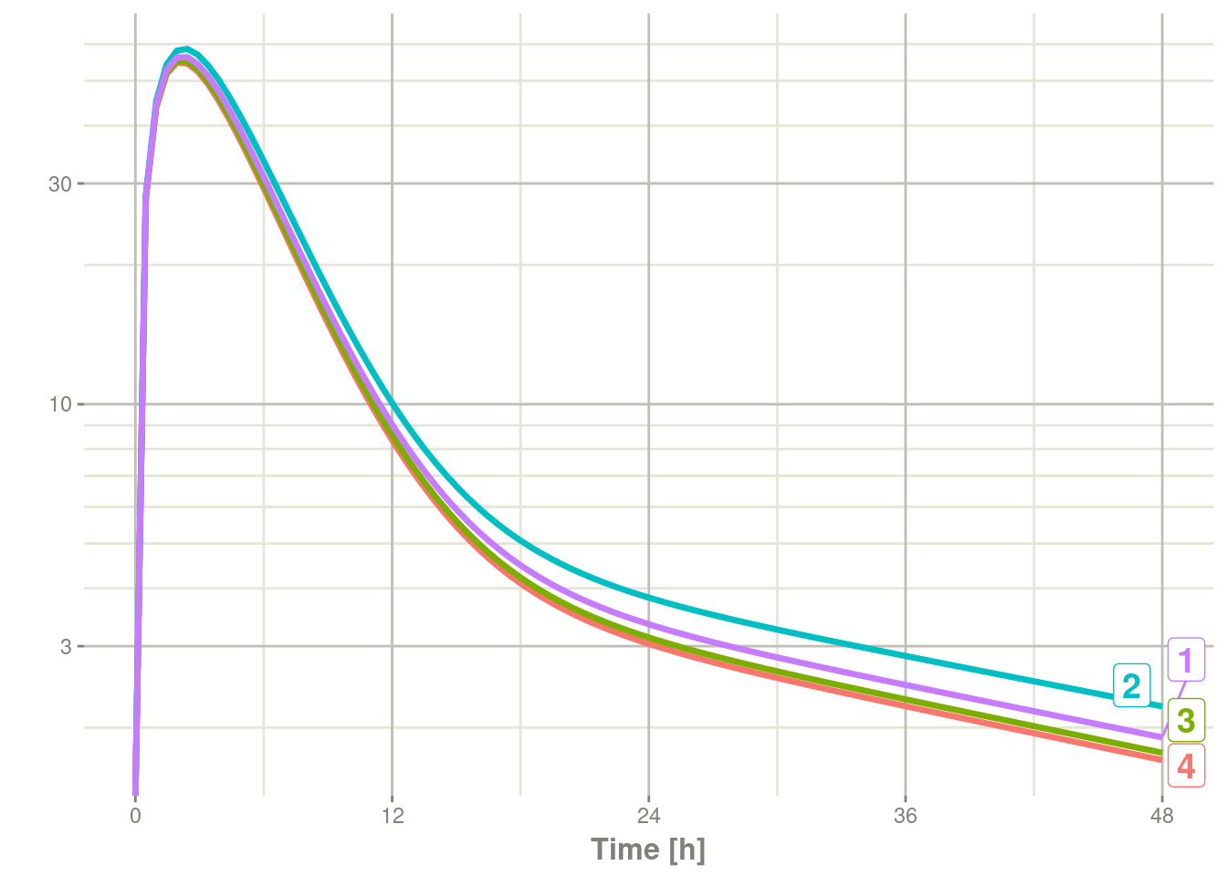

13.1.2 Time Varying Covariates

Covariates are easy to specify in RxODE, you can specify them as a variable. Time-varying covariates, like clock time in a circadian rhythm model, can also be used. Extending the indirect response model already discussed, we have:

library(RxODE)
library(units)

mod3 <- RxODE({
    KA=2.94E-01;
    CL=1.86E+01;
    V2=4.02E+01;
    Q=1.05E+01;
    V3=2.97E+02;
    Kin0=1;
    Kout=1;
    EC50=200;
#### The linCmt() picks up the variables from above
    C2   = linCmt();
    Tz= 8
    amp=0.1
    eff(0) = 1  ## This specifies that the effect compartment starts at 1.
#### Kin changes based on time of day (like cortosol)
    Kin =   Kin0 +amp *cos(2*pi*(ctime-Tz)/24)
    d/dt(eff) =  Kin - Kout*(1-C2/(EC50+C2))*eff;
})


ev <- eventTable(amount.units="mg", time.units="hours") %>%
    add.dosing(dose=10000, nbr.doses=1, dosing.to=1) %>%
    add.sampling(seq(0,48,length.out=100));


#### Create data frame of 8 am dosing for the first dose This is done
#### with base R but it can be done with dplyr or data.table
ev$ctime <- (ev$time+set_units(8,hr)) %% 24

Now there is a covariate present in the event dataset, the system can be solved by combining the dataset and the model:

r1 <- solve(mod3, ev, covs_interpolation="linear")
print(r1)
#> ______________________________ Solved RxODE object _____________________________
#> -- Parameters ($params): -------------------------------------------------------
#>         KA         CL         V2          Q         V3       Kin0       Kout 
#>   0.294000  18.600000  40.200000  10.500000 297.000000   1.000000   1.000000 
#>       EC50         Tz        amp         pi 
#> 200.000000   8.000000   0.100000   3.141593 
#> -- Initial Conditions ($inits): ------------------------------------------------
#> eff 
#>   1 
#> -- First part of data (object): ------------------------------------------------
#> # A tibble: 100 x 4
#>        time    C2   Kin   eff
#>         [h] <dbl> <dbl> <dbl>
#> 1 0.0000000   0    1.1   1   
#> 2 0.4848485  27.8  1.10  1.07
#> 3 0.9696970  43.7  1.10  1.15
#> 4 1.4545455  51.8  1.09  1.22
#> 5 1.9393939  54.8  1.09  1.27
#> 6 2.4242424  54.6  1.08  1.30
#> # ... with 94 more rows
#> ________________________________________________________________________________

When solving ODE equations, the solver may sample times outside of the data. When this happens, this ODE solver can use linear interpolation between the covariate values. It is equivalent to R’s approxfun with method="linear".

plot(r1,C2, ylab="Central Concentration")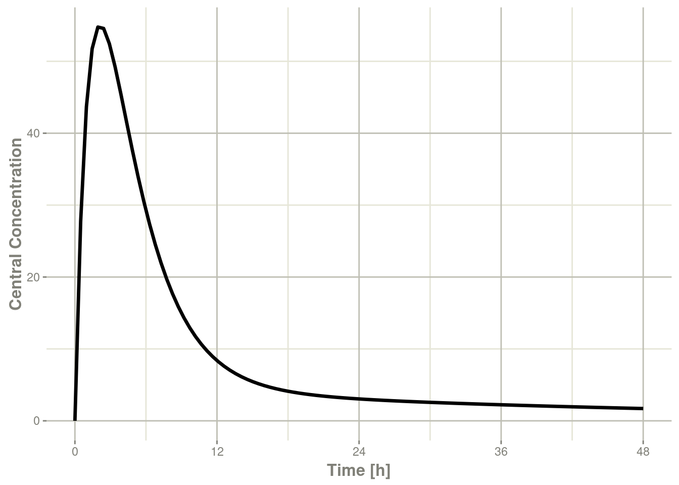

plot(r1,eff) + ylab("Effect") + xlab("Time");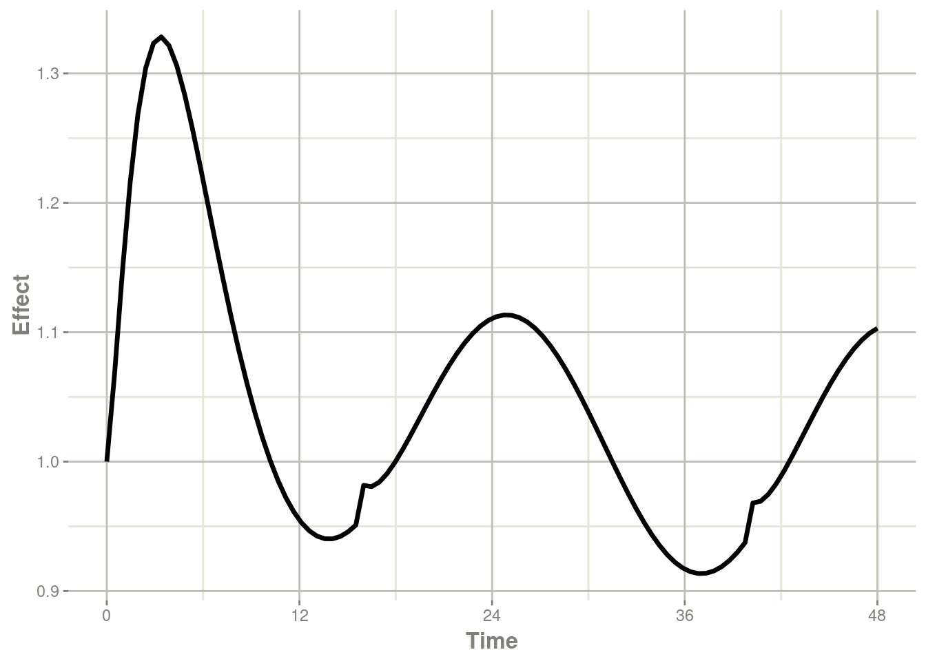

Note that the linear approximation in this case leads to some kinks in the solved system at 24-hours where the covariate has a linear interpolation between near 24 and near 0. While linear seems reasonable, cases like clock time make other interpolation methods more attractive.

In RxODE the default covariate interpolation is be the last observation carried forward (locf), or constant approximation. This is equivalent to R’s approxfun with method="constant".

r1 <- solve(mod3, ev,covs_interpolation="constant")
print(r1)
#> ______________________________ Solved RxODE object _____________________________
#> -- Parameters ($params): -------------------------------------------------------
#>         KA         CL         V2          Q         V3       Kin0       Kout 
#>   0.294000  18.600000  40.200000  10.500000 297.000000   1.000000   1.000000 
#>       EC50         Tz        amp         pi 
#> 200.000000   8.000000   0.100000   3.141593 
#> -- Initial Conditions ($inits): ------------------------------------------------
#> eff 
#>   1 
#> -- First part of data (object): ------------------------------------------------
#> # A tibble: 100 x 4
#>        time    C2   Kin   eff
#>         [h] <dbl> <dbl> <dbl>
#> 1 0.0000000   0    1.1   1   
#> 2 0.4848485  27.8  1.10  1.07
#> 3 0.9696970  43.7  1.10  1.15
#> 4 1.4545455  51.8  1.09  1.22
#> 5 1.9393939  54.8  1.09  1.27
#> 6 2.4242424  54.6  1.08  1.31
#> # ... with 94 more rows
#> ________________________________________________________________________________

which gives the following plots:

plot(r1,C2, ylab="Central Concentration", xlab="Time")

plot(r1,eff, ylab="Effect", xlab="Time")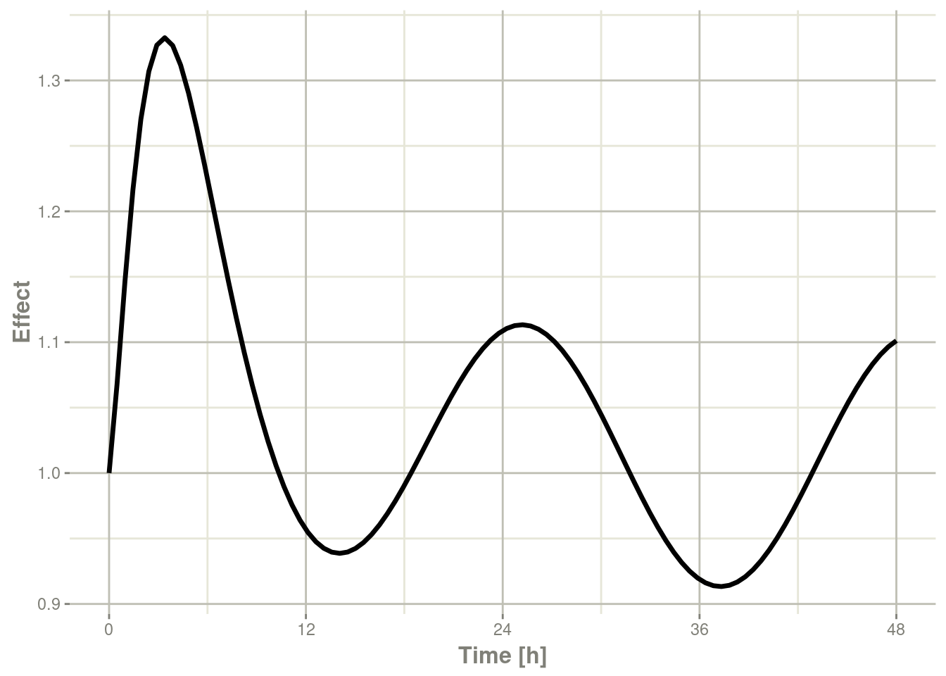

In this case, the plots seem to be smoother.

You can also use NONMEM’s preferred interpolation style of next observation carried backward (NOCB):

r1 <- solve(mod3, ev,covs_interpolation="nocb")
print(r1)
#> ______________________________ Solved RxODE object _____________________________
#> -- Parameters ($params): -------------------------------------------------------
#>         KA         CL         V2          Q         V3       Kin0       Kout 
#>   0.294000  18.600000  40.200000  10.500000 297.000000   1.000000   1.000000 
#>       EC50         Tz        amp         pi 
#> 200.000000   8.000000   0.100000   3.141593 
#> -- Initial Conditions ($inits): ------------------------------------------------
#> eff 
#>   1 
#> -- First part of data (object): ------------------------------------------------
#> # A tibble: 100 x 4
#>        time    C2   Kin   eff
#>         [h] <dbl> <dbl> <dbl>
#> 1 0.0000000   0    1.1   1   
#> 2 0.4848485  27.8  1.10  1.07
#> 3 0.9696970  43.7  1.10  1.15
#> 4 1.4545455  51.8  1.09  1.21
#> 5 1.9393939  54.8  1.09  1.27
#> 6 2.4242424  54.6  1.08  1.30
#> # ... with 94 more rows
#> ________________________________________________________________________________

which gives the following plots:

plot(r1,C2, ylab="Central Concentration", xlab="Time")

plot(r1,eff, ylab="Effect", xlab="Time")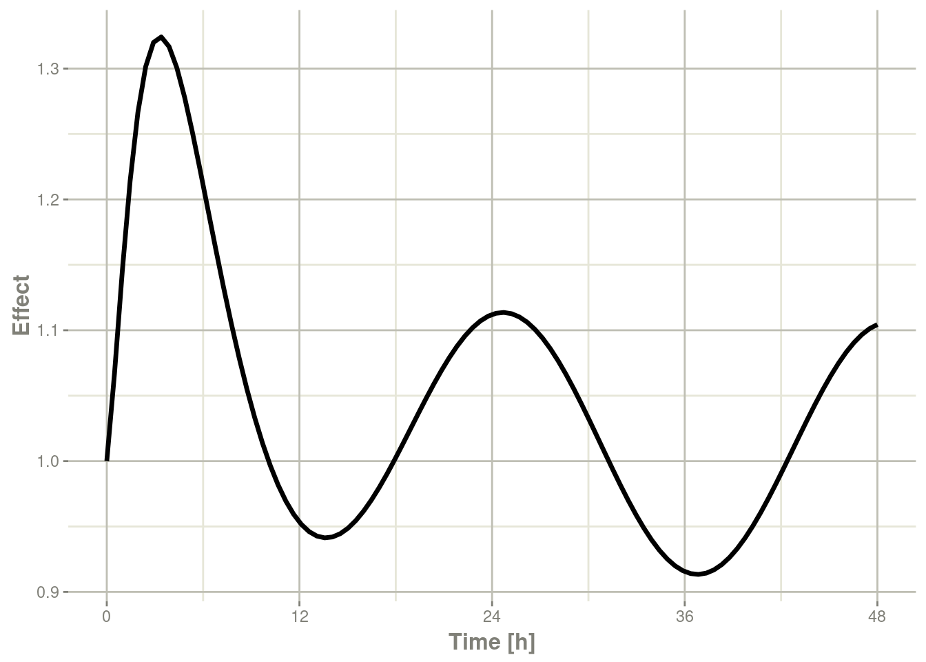

13.2 Shiny and RxODE

13.2.1 Facilities for generating R shiny applications

An example of creating an R shiny application to interactively explore responses of various complex dosing regimens is available at http://qsp.engr.uga.edu:3838/RxODE/RegimenSimulator. Shiny applications like this one may be programmatically created with the experimental function genShinyApp.template().

The above application includes widgets for varying the dose, dosing regimen, dose cycle, and number of cycles.

genShinyApp.template(appDir = "shinyExample", verbose=TRUE)

library(shiny)
runApp("shinyExample")

Click here to go to the Shiny App

13.2.2 Exploring parameter fits graphically using shiny

An RxODE object can be explored with rxShiny(obj). rxShiny() will also allow you to try new models to see how they behave.

13.3 Using RxODE with a pipeline

13.3.1 Setting up the RxODE model for the pipeline

In this example we will show how to use RxODE in a simple pipeline.

We can start with a model that can be used for the different simulation workflows that RxODE can handle:

library(RxODE)

Ribba2012 <- RxODE({
    k = 100

    tkde = 0.24
    eta.tkde = 0
    kde ~ tkde*exp(eta.tkde)

    tkpq = 0.0295
    eta.kpq = 0
    kpq ~ tkpq * exp(eta.kpq)

    tkqpp = 0.0031
    eta.kqpp = 0
    kqpp ~ tkqpp * exp(eta.kqpp)

    tlambdap = 0.121
    eta.lambdap = 0
    lambdap ~ tlambdap*exp(eta.lambdap)

    tgamma = 0.729
    eta.gamma = 0
    gamma ~ tgamma*exp(eta.gamma)

    tdeltaqp = 0.00867
    eta.deltaqp = 0
    deltaqp ~ tdeltaqp*exp(eta.deltaqp)

    prop.err <- 0
    pstar <- (pt+q+qp)*(1+prop.err)
    d/dt(c) = -kde * c
    d/dt(pt) = lambdap * pt *(1-pstar/k) + kqpp*qp -
        kpq*pt - gamma*c*kde*pt
    d/dt(q) = kpq*pt -gamma*c*kde*q
    d/dt(qp) = gamma*c*kde*q - kqpp*qp - deltaqp*qp
#### initial conditions
    tpt0 = 7.13
    eta.pt0 = 0
    pt0 ~ tpt0*exp(eta.pt0)
    tq0 = 41.2
    eta.q0 = 0
    q0 ~ tq0*exp(eta.q0)
    pt(0) = pt0
    q(0) = q0
})

This is a tumor growth model described in Ribba 2012. In this case, we compiled the model into an R object Ribba2012, though in an RxODE simulation pipeline, you do not have to assign the compiled model to any object, though I think it makes sense.

13.3.2 Simulating one event table

Simulating a single event table is quite simple:

• You pipe the RxODE simulation object into an event table object by et().
  
• When the events are completely specified, you simply solve the ODE system with rxSolve().
• In this case you can pipe the output to plot() to conveniently view the results.
• Note for the plot we are only selecting the selecting following:
  • pt (Proliferative Tissue),
  • q (quiescent tissue)
  • qp (DNA-Damaged quiescent tissue) and
  • pstar (total tumor tissue)

Ribba2012 %>% # Use RxODE
    et(time.units="months") %>% # Pipe to a new event table
    et(amt=1, time=50, until=58, ii=1.5) %>% # Add dosing every 1.5 months
    et(0, 250, by=0.5) %>% # Add some sampling times (not required)
    rxSolve() %>% # Solve the simulation
    plot(pt, q, qp, pstar) # Plot it, plotting the variables of interest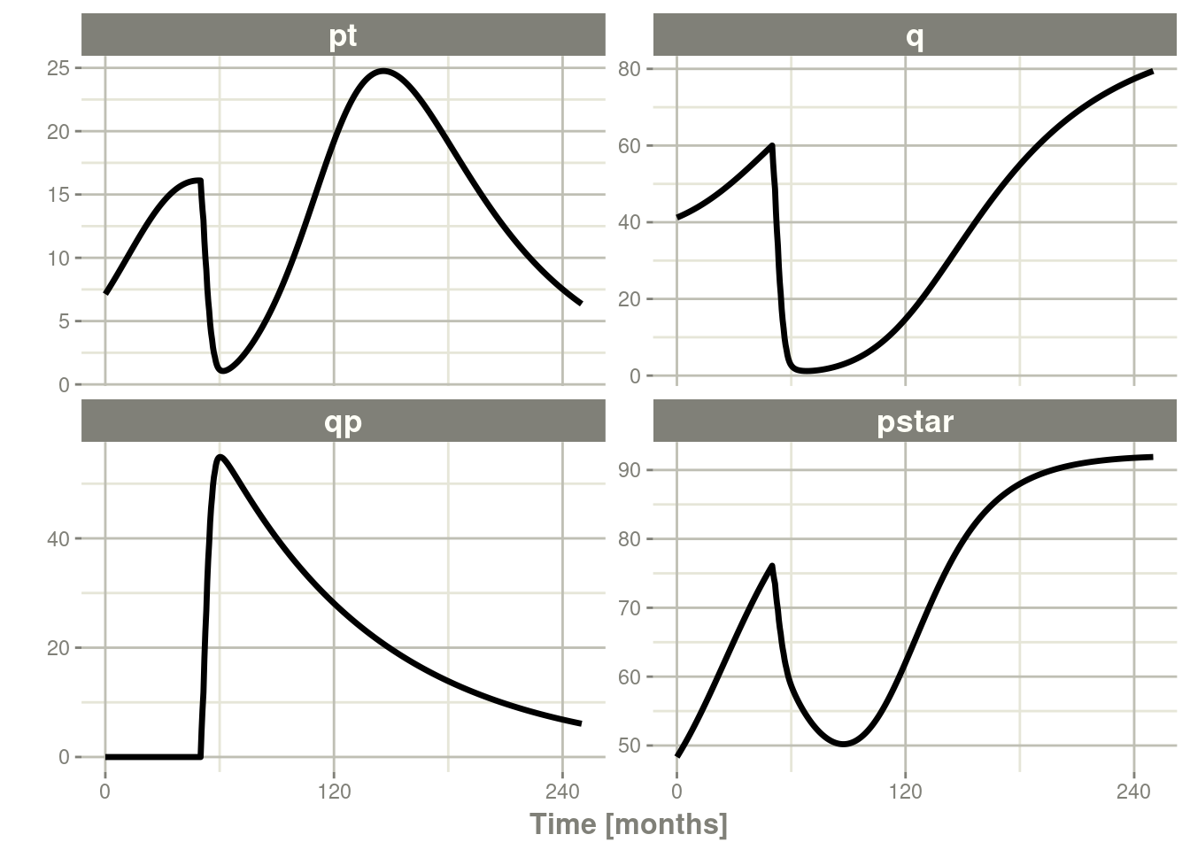

13.3.3 Simulating multiple subjects from a single event table

13.3.3.1 Simulating with between subject variability

The next sort of simulation that may be useful is simulating multiple patients with the same treatments. In this case, we will use the omega matrix specified by the paper:

#### Add CVs from paper for individual simulation
#### Uses exact formula:

lognCv = function(x){log((x/100)^2+1)}

library(lotri)
#### Now create omega matrix
#### I'm using lotri to quickly specify names/diagonals
omega <- lotri(eta.pt0 ~ lognCv(94),
               eta.q0 ~ lognCv(54),
               eta.lambdap ~ lognCv(72),
               eta.kqp ~ lognCv(76),
               eta.qpp ~ lognCv(97),
               eta.deltaqp ~ lognCv(115),
               eta.kde ~ lognCv(70))

omega
#>               eta.pt0    eta.q0 eta.lambdap   eta.kqp   eta.qpp eta.deltaqp
#> eta.pt0     0.6331848 0.0000000   0.0000000 0.0000000 0.0000000   0.0000000
#> eta.q0      0.0000000 0.2558818   0.0000000 0.0000000 0.0000000   0.0000000
#> eta.lambdap 0.0000000 0.0000000   0.4176571 0.0000000 0.0000000   0.0000000
#> eta.kqp     0.0000000 0.0000000   0.0000000 0.4559047 0.0000000   0.0000000
#> eta.qpp     0.0000000 0.0000000   0.0000000 0.0000000 0.6631518   0.0000000
#> eta.deltaqp 0.0000000 0.0000000   0.0000000 0.0000000 0.0000000   0.8426442
#> eta.kde     0.0000000 0.0000000   0.0000000 0.0000000 0.0000000   0.0000000
#>               eta.kde
#> eta.pt0     0.0000000
#> eta.q0      0.0000000
#> eta.lambdap 0.0000000
#> eta.kqp     0.0000000
#> eta.qpp     0.0000000
#> eta.deltaqp 0.0000000
#> eta.kde     0.3987761

With this information, it is easy to simulate 3 subjects from the model-based parameters:

set.seed(1089)
Ribba2012 %>% # Use RxODE
    et(time.units="months") %>% # Pipe to a new event table
    et(amt=1, time=50, until=58, ii=1.5) %>% # Add dosing every 1.5 months
    et(0, 250, by=0.5) %>% # Add some sampling times (not required)
    rxSolve(nSub=3, omega=omega) %>% # Solve the simulation
    plot(pt, q, qp, pstar) # Plot it, plotting the variables of interest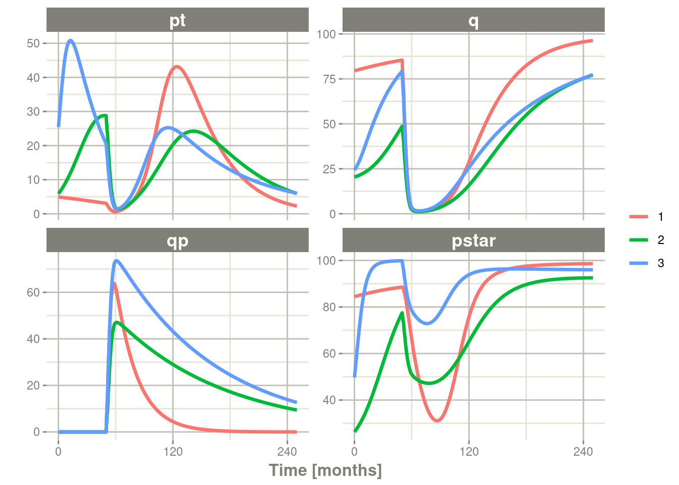

Note there are two different things that were added to this simulation: - nSub to specify how many subjects are in the model - omega to specify the between subject variability.

13.3.3.2 Simulation with unexplained variability

You can even add unexplained variability quite easily:

Ribba2012 %>% # Use RxODE
    et(time.units="months") %>% # Pipe to a new event table
    et(amt=1, time=50, until=58, ii=1.5) %>% # Add dosing every 1.5 months
     et(0, 250, by=0.5) %>% # Add some sampling times (not required)
    rxSolve(nSub=3, omega=omega, sigma=lotri(prop.err ~ 0.05^2)) %>% # Solve the simulation
    plot(pt, q, qp, pstar) # Plot it, plotting the variables of interest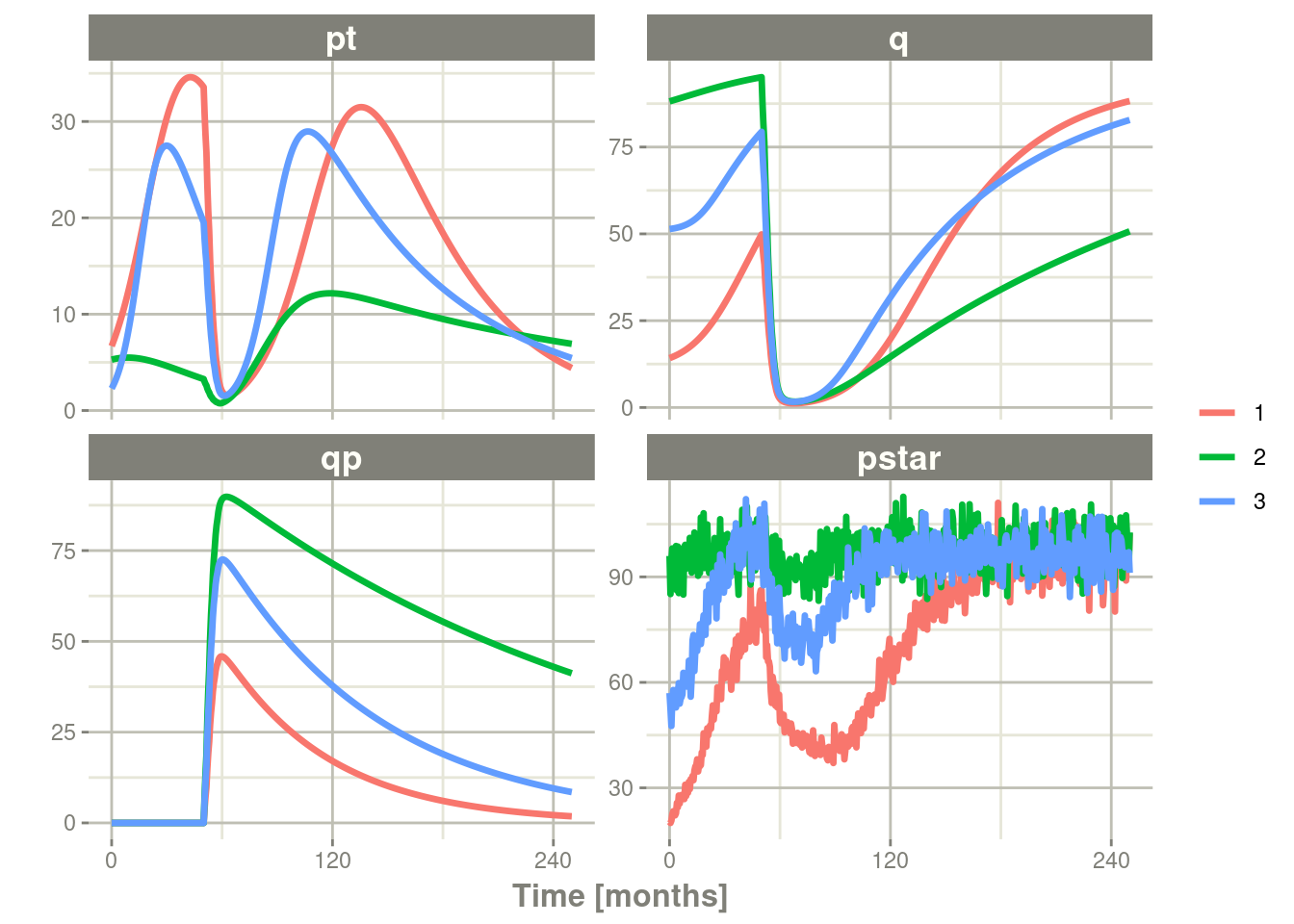

In this case we only added the sigma matrix to have unexplained variability on the pstar or total tumor tissue.

You can even simulate with uncertainty in the theta omega and sigma values if you wish.

13.3.3.3 Simulation with uncertainty in all the parameters (by matrices)

If we assume these parameters came from 95 subjects with 8 observations apiece, the degrees of freedom for the omega matrix would be 95, and the degrees of freedom of the sigma matrix would be 95*8=760 because 95 items informed the omega matrix, and 760 items informed the sigma matrix.

Ribba2012 %>% # Use RxODE
    et(time.units="months") %>% # Pipe to a new event table
    et(amt=1, time=50, until=58, ii=1.5) %>% # Add dosing every 1.5 months
    et(0, 250, by=0.5) %>% # Add some sampling times (not required)
    rxSolve(nSub=3, nStud=3, omega=omega, sigma=lotri(prop.err ~ 0.05^2),
            dfSub=760, dfObs=95) %>% # Solve the simulation
    plot(pt, q, qp, pstar) # Plot it, plotting the variables of interest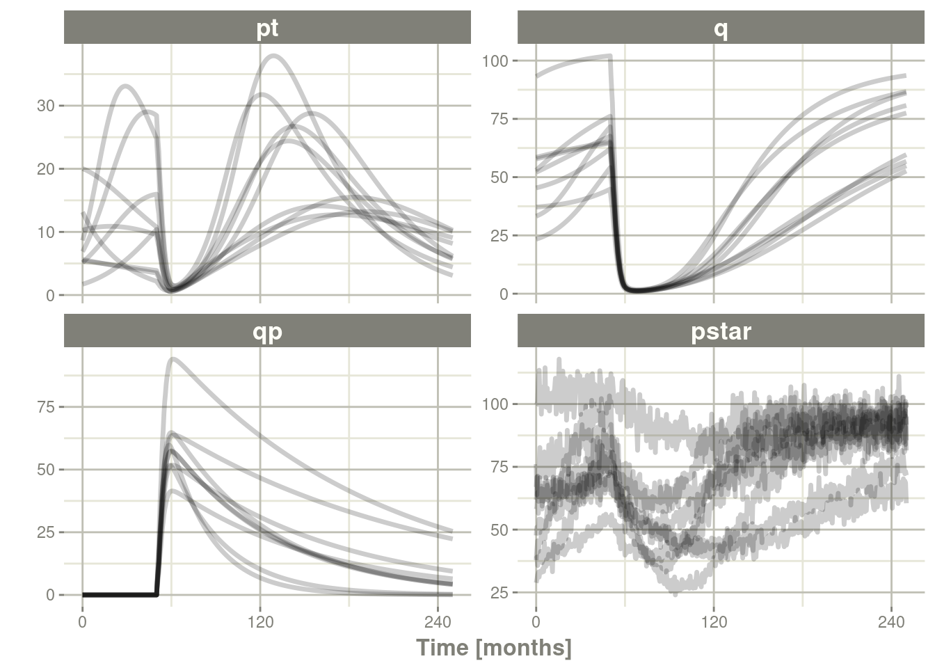

Often in simulations we have a full covariance matrix for the fixed effect parameters. In this case, we do not have the matrix, but it could be specified by thetaMat.

While we do not have a full covariance matrix, we can have information about the diagonal elements of the covariance matrix from the model paper. These can be converted as follows:

rseVar <- function(est, rse){
    return(est*rse/100)^2
}

thetaMat <- lotri(tpt0 ~ rseVar(7.13,25),
                  tq0 ~ rseVar(41.2,7),
                  tlambdap ~ rseVar(0.121, 16),
                  tkqpp ~ rseVar(0.0031, 35),
                  tdeltaqp ~ rseVar(0.00867, 21),
                  tgamma ~ rseVar(0.729, 37),
                  tkde ~ rseVar(0.24, 33)
                  );

thetaMat
#>            tpt0   tq0 tlambdap    tkqpp  tdeltaqp  tgamma   tkde
#> tpt0     1.7825 0.000  0.00000 0.000000 0.0000000 0.00000 0.0000
#> tq0      0.0000 2.884  0.00000 0.000000 0.0000000 0.00000 0.0000
#> tlambdap 0.0000 0.000  0.01936 0.000000 0.0000000 0.00000 0.0000
#> tkqpp    0.0000 0.000  0.00000 0.001085 0.0000000 0.00000 0.0000
#> tdeltaqp 0.0000 0.000  0.00000 0.000000 0.0018207 0.00000 0.0000
#> tgamma   0.0000 0.000  0.00000 0.000000 0.0000000 0.26973 0.0000
#> tkde     0.0000 0.000  0.00000 0.000000 0.0000000 0.00000 0.0792

Now we have a thetaMat to represent the uncertainty in the theta matrix, as well as the other pieces in the simulation. Typically you can put this information into your simulation with the thetaMat matrix.

With such large variability in theta it is easy to sample a negative rate constant, which does not make sense. For example:

Ribba2012 %>% # Use RxODE
et(time.units="months") %>% # Pipe to a new event table
et(amt=1, time=50, until=58, ii=1.5) %>% # Add dosing every 1.5 months
et(0, 250, by=0.5) %>% # Add some sampling times (not required)
rxSolve(nSub=2, nStud=2, omega=omega, sigma=lotri(prop.err ~ 0.05^2),
thetaMat=thetaMat, 
dfSub=760, dfObs=95) %>% # Solve the simulation
plot(pt, q, qp, pstar) # Plot it, plotting the variables of interest

#> unhandled error message: EE:[lsoda] 70000 steps taken before reaching tout
#> @(lsoda.c:750
#> Warning message:
#> In rxSolve_(object, .ctl, .nms, .xtra, params, events, inits, setupOnly = .setupOnly) :
#>  Some ID(s) could not solve the ODEs correctly; These values are replaced with NA.

To correct these problems you simply need to use a truncated multivariate normal and specify the reasonable ranges for the parameters. For theta this is specified by thetaLower and thetaUpper. Similar parameters are there for the other matrices: omegaLower, omegaUpper, sigmaLower and sigmaUpper. These may be named vectors, one numeric value, or a numeric vector matching the number of parameters specified in the thetaMat matrix.

In this case the simulation simply has to be modified to have thetaLower=0 to make sure all rates are positive:

Ribba2012 %>% # Use RxODE
    et(time.units="months") %>% # Pipe to a new event table
    et(amt=1, time=50, until=58, ii=1.5) %>% # Add dosing every 1.5 months
    et(0, 250, by=0.5) %>% # Add some sampling times (not required)
    rxSolve(nSub=2, nStud=2, omega=omega, sigma=lotri(prop.err ~ 0.05^2),
            thetaMat=thetaMat,
            thetaLower=0, # Make sure the rates are reasonable
            dfSub=760, dfObs=95) %>% # Solve the simulation
    plot(pt, q, qp, pstar) # Plot it, plotting the variables of interest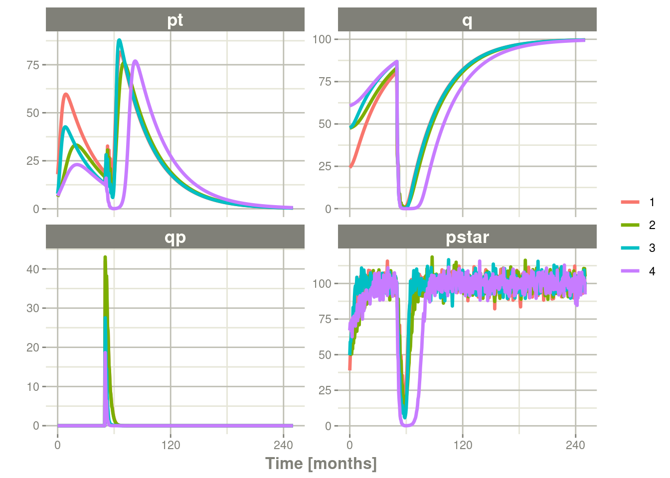

13.3.4 Summarizing the simulation output

While it is easy to use dplyr and data.table to perform your own summary of simulations, RxODE also provides this ability by the confint function.

#### This takes a little more time; Most of the time is the summary
#### time.

sim0 <- Ribba2012 %>% # Use RxODE
    et(time.units="months") %>% # Pipe to a new event table
    et(amt=1, time=50, until=58, ii=1.5) %>% # Add dosing every 1.5 months
    et(0, 250, by=0.5) %>% # Add some sampling times (not required)
    rxSolve(nSub=10, nStud=10, omega=omega, sigma=lotri(prop.err ~ 0.05^2),
            thetaMat=thetaMat,
            thetaLower=0, # Make sure the rates are reasonable
            dfSub=760, dfObs=95) %>% # Solve the simulation
    confint(c("pt","q","qp","pstar"),level=0.90); # Create Simulation intervals

sim0 %>% plot() # Plot the simulation intervals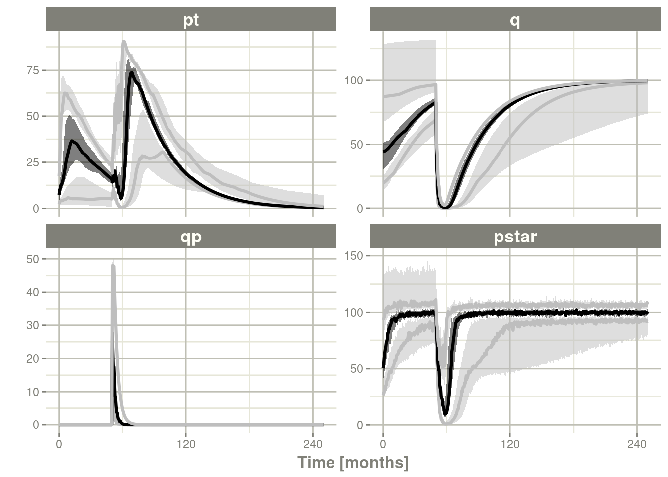

13.3.4.1 Simulating from a data-frame of parameters

While the simulation from matrices can be very useful and a fast way to simulate information, sometimes you may want to simulate more complex scenarios. For instance, there may be some reason to believe that tkde needs to be above tlambdap, therefore these need to be simulated more carefully. You can generate the data frame in whatever way you want. The internal method of simulating the new parameters is exported too.

library(dplyr)
pars <- rxInits(Ribba2012);
pars <- pars[regexpr("(prop|eta)",names(pars)) == -1]
print(pars)
#>        k     tkde     tkpq    tkqpp tlambdap   tgamma tdeltaqp     tpt0 
#> 1.00e+02 2.40e-01 2.95e-02 3.10e-03 1.21e-01 7.29e-01 8.67e-03 7.13e+00 
#>      tq0 
#> 4.12e+01
#### This is the exported method for simulation of Theta/Omega internally in RxODE
df <- rxSimThetaOmega(params=pars, omega=omega,dfSub=760,
                      thetaMat=thetaMat, thetaLower=0, nSub=60,nStud=60) %>%
    filter(tkde > tlambdap) %>% as.tbl()
#### You could also simulate more and bind them together to a data frame.
print(df)
#> # A tibble: 2,340 x 16
#>        k  tkde   tkpq tkqpp tlambdap tgamma tdeltaqp  tpt0   tq0 eta.pt0 eta.q0
#>    <dbl> <dbl>  <dbl> <dbl>    <dbl>  <dbl>    <dbl> <dbl> <dbl>   <dbl>  <dbl>
#>  1   100  2.83 0.0295 0.239    0.683  0.861     1.25  7.67  42.0  0.559   0.136
#>  2   100  2.83 0.0295 0.239    0.683  0.861     1.25  7.67  42.0  0.0465 -0.581
#>  3   100  2.83 0.0295 0.239    0.683  0.861     1.25  7.67  42.0 -0.188  -0.180
#>  4   100  2.83 0.0295 0.239    0.683  0.861     1.25  7.67  42.0  0.321   0.614
#>  5   100  2.83 0.0295 0.239    0.683  0.861     1.25  7.67  42.0  0.0656 -0.232
#>  6   100  2.83 0.0295 0.239    0.683  0.861     1.25  7.67  42.0  0.0194  0.517
#>  7   100  2.83 0.0295 0.239    0.683  0.861     1.25  7.67  42.0 -0.218   0.260
#>  8   100  2.83 0.0295 0.239    0.683  0.861     1.25  7.67  42.0 -0.258  -0.761
#>  9   100  2.83 0.0295 0.239    0.683  0.861     1.25  7.67  42.0 -1.28   -1.34 
#> 10   100  2.83 0.0295 0.239    0.683  0.861     1.25  7.67  42.0 -0.495   0.161
#> # ... with 2,330 more rows, and 5 more variables: eta.lambdap <dbl>,
#> #   eta.kqp <dbl>, eta.qpp <dbl>, eta.deltaqp <dbl>, eta.kde <dbl>
#### Quick check to make sure that all the parameters are OK.
all(df$tkde>df$tlambdap)
#> [1] TRUE
sim1 <- Ribba2012 %>% # Use RxODE
    et(time.units="months") %>% # Pipe to a new event table
    et(amt=1, time=50, until=58, ii=1.5) %>% # Add dosing every 1.5 months
    et(0, 250, by=0.5) %>% # Add some sampling times (not required)
    rxSolve(df)
#### Note this information looses information about which ID is in a
#### "study", so it summarizes the confidence intervals by dividing the
#### subjects into sqrt(#subjects) subjects and then summarizes the
#### confidence intervals
sim2 <- sim1 %>% confint(c("pt","q","qp","pstar"),level=0.90); # Create Simulation intervals
save(sim2, file = file.path(system.file(package = "RxODE"), "pipeline-sim2.rds"), version = 2)
sim2 %>% plot()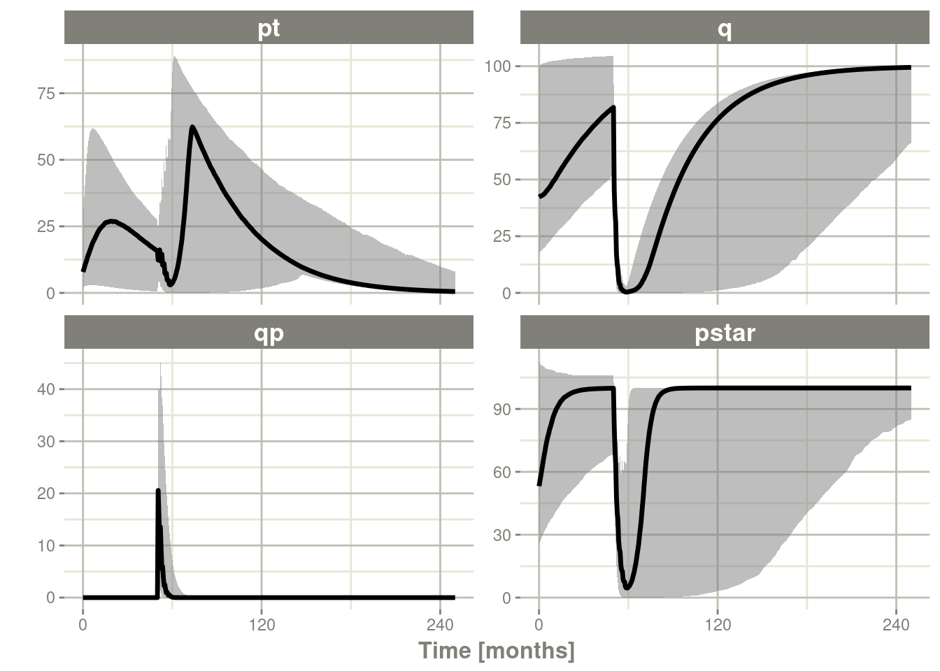

13.4 Speeding up RxODE

13.4.1 Increasing RxODE speed by multi-subject parallel solving

RxODE originally developed as an ODE solver that allowed an ODE solve for a single subject. This flexibility is still supported.

The original code from the RxODE tutorial is below:

library(RxODE)

library(microbenchmark)
library(ggplot2)

mod1 <- RxODE({
    C2 = centr/V2;
    C3 = peri/V3;
    d/dt(depot) = -KA*depot;
    d/dt(centr) = KA*depot - CL*C2 - Q*C2 + Q*C3;
    d/dt(peri) = Q*C2 - Q*C3;
    d/dt(eff) = Kin - Kout*(1-C2/(EC50+C2))*eff;
    eff(0) = 1
})

#### Create an event table

ev <- et() %>%
    et(amt=10000, addl=9,ii=12) %>%
    et(time=120, amt=20000, addl=4, ii=24) %>%
    et(0:240) ## Add Sampling

nsub <- 100 # 100 sub-problems
sigma <- matrix(c(0.09,0.08,0.08,0.25),2,2) # IIV covariance matrix
mv <- rxRmvn(n=nsub, rep(0,2), sigma) # Sample from covariance matrix
CL <- 7*exp(mv[,1])
V2 <- 40*exp(mv[,2])
params.all <- cbind(KA=0.3, CL=CL, V2=V2, Q=10, V3=300,
                    Kin=0.2, Kout=0.2, EC50=8)

13.4.1.1 For Loop

The slowest way to code this is to use a for loop. In this example we will enclose it in a function to compare timing.

runFor <- function(){
    res <- NULL
    for (i in 1:nsub) {
        params <- params.all[i,]
        x <- mod1$solve(params, ev, cacheEvent=FALSE)
        ##Store results for effect compartment
        res <- cbind(res, x[, "eff"])
    }
    return(res)
}

13.4.1.2 Running with apply

In general for R, the apply types of functions perform better than a for loop, so the tutorial also suggests this speed enhancement

runSapply <- function(){
    res <- apply(params.all, 1, function(theta)
        mod1$run(theta, ev, cacheEvent=FALSE)[, "eff"])
}

13.4.1.3 Run using a single-threaded solve

You can also have RxODE solve all the subject simultaneously without collecting the results in R, using a single threaded solve.

The data output is slightly different here, but still gives the same information:

runSingleThread <- function(){
    solve(mod1, params.all, ev, cores=1, cacheEvent=FALSE)[,c("sim.id", "time", "eff")]
}

13.4.1.4 Run a 2 threaded solve

RxODE supports multi-threaded solves, so another option is to have 2 threads (called cores in the solve options, you can see the options in rxControl() or rxSolve()).

run2Thread <- function(){
    solve(mod1, params.all, ev, cores=2, cacheEvent=FALSE)[,c("sim.id", "time", "eff")]
}

13.4.1.5 Compare the times between all the methods

Now the moment of truth, the timings:

bench <- microbenchmark(runFor(), runSapply(), runSingleThread(),run2Thread())
print(bench)
#> Unit: milliseconds
#>               expr       min        lq      mean    median        uq       max
#>           runFor() 149.52081 171.27062 192.90942 190.02686 211.04242 349.87083
#>        runSapply() 148.46279 170.85325 192.90897 203.24540 209.75845 343.35761
#>  runSingleThread()  21.79790  25.92407  27.43815  26.63215  29.40284  34.89256
#>       run2Thread()  13.99345  15.03455  16.58391  15.26519  15.79007  32.19146
#>  neval
#>    100
#>    100
#>    100
#>    100
autoplot(bench)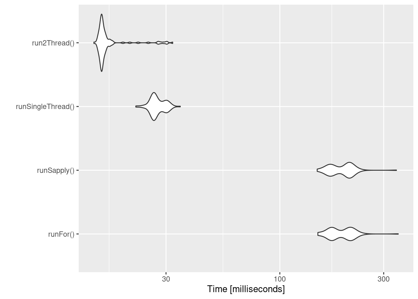

It is clear that the largest jump in performance when using the solve method and providing all the parameters to RxODE to solve without looping over each subject with either a for or a sapply. The number of cores/threads applied to the solve also plays a role in the solving.

We can explore the number of threads further with the following code:

runThread <- function(n){
    solve(mod1, params.all, ev, cores=n, cacheEvent=FALSE)[,c("sim.id", "time", "eff")]
}

bench <- eval(parse(text=sprintf("microbenchmark(%s)",
                                     paste(paste0("runThread(", seq(1, 2 * rxCores()),")"),
                                           collapse=","))))
print(bench)
#> Unit: milliseconds
#>          expr      min       lq     mean    median        uq       max neval
#>  runThread(1) 21.50871 23.13192 39.27643  25.81496  27.56073 1021.6726   100
#>  runThread(2) 13.14395 14.72681 44.98351  16.65848  29.15620  814.2002   100
#>  runThread(3) 11.38847 12.71787 48.01460  19.05276  21.92472  446.1831   100
#>  runThread(4) 14.65711 16.10307 54.13006  16.70819  20.03974  411.9033   100
#>  runThread(5) 12.95509 14.35766 57.15010  15.32234  20.12732  433.2323   100
#>  runThread(6) 12.62878 13.48153 62.76636  13.98110  22.89068  475.2186   100
#>  runThread(7) 11.52002 12.94464 70.78100  14.47153 132.10935  522.5479   100
#>  runThread(8) 21.04313 32.49421 92.58168 106.31139 131.07819  370.4774   100
autoplot(bench)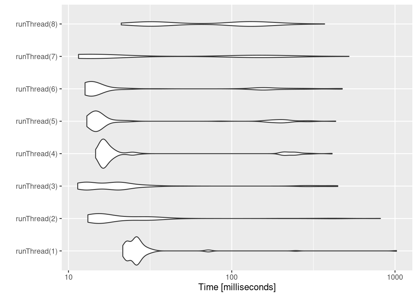

There can be a suite spot in speed vs number or cores. The system type (mac, linux, windows and/or processor), complexity of the ODE solving and the number of subjects may affect this arbitrary number of threads. 4 threads is a good number to use without any prior knowledge because most systems these days have at least 4 threads (or 2 processors with 4 threads).

13.4.2 A real life example

Before some of the parallel solving was implemented, the fastest way to run RxODE was with lapply. This is how Rik Schoemaker created the data-set for nlmixr comparisons, but reduced to run faster automatic building of the pkgdown website.

library(RxODE)
library(data.table)
#Define the RxODE model
  ode1 <- "
  d/dt(abs)    = -KA*abs;
  d/dt(centr)  =  KA*abs-(CL/V)*centr;
  C2=centr/V;
  "
  
#Create the RxODE simulation object
mod1 <- RxODE(model = ode1)

#Population parameter values on log-scale
  paramsl <- c(CL = log(4),
               V = log(70),
               KA = log(1))
#make 10,000 subjects to sample from:
  nsubg <- 300 # subjects per dose
  doses <- c(10, 30, 60, 120)
  nsub <- nsubg * length(doses)
#IIV of 30% for each parameter
  omega <- diag(c(0.09, 0.09, 0.09))# IIV covariance matrix
  sigma <- 0.2
#Sample from the multivariate normal
  set.seed(98176247)
  library(MASS)
  mv <-
    mvrnorm(nsub, rep(0, dim(omega)[1]), omega) # Sample from covariance matrix
#Combine population parameters with IIV
  params.all <-
    data.table(
      "ID" = seq(1:nsub),
      "CL" = exp(paramsl['CL'] + mv[, 1]),
      "V" = exp(paramsl['V'] + mv[, 2]),
      "KA" = exp(paramsl['KA'] + mv[, 3])
    )
#set the doses (looping through the 4 doses)
params.all[, AMT := rep(100 * doses,nsubg)]

Startlapply <- Sys.time()
  
#Run the simulations using lapply for speed
  s = lapply(1:nsub, function(i) {
#selects the parameters associated with the subject to be simulated
    params <- params.all[i]
#creates an eventTable with 7 doses every 24 hours
    ev <- eventTable()
    ev$add.dosing(
      dose = params$AMT,
      nbr.doses = 1,
      dosing.to = 1,
      rate = NULL,
      start.time = 0
    )
#generates 4 random samples in a 24 hour period
    ev$add.sampling(c(0, sort(round(sample(runif(600, 0, 1440), 4) / 60, 2))))
#runs the RxODE simulation
    x <- as.data.table(mod1$run(params, ev))
#merges the parameters and ID number to the simulation output
    x[, names(params) := params]
  })
  
#runs the entire sequence of 100 subjects and binds the results to the object res
  res = as.data.table(do.call("rbind", s))
  
Stoplapply <- Sys.time()
  
print(Stoplapply - Startlapply)
#> Time difference of 6.183588 secs

By applying some of the new parallel solving concepts you can simply run the same simulation both with less code and faster:

rx <- RxODE({
    CL =  log(4)
    V = log(70)
    KA = log(1)
    CL = exp(CL + eta.CL)
    V = exp(V + eta.V)
    KA = exp(KA + eta.KA)
    d/dt(abs)    = -KA*abs;
    d/dt(centr)  =  KA*abs-(CL/V)*centr;
    C2=centr/V;
})

omega <- lotri(eta.CL ~ 0.09,
               eta.V ~ 0.09,
               eta.KA ~ 0.09)

doses <- c(10, 30, 60, 120)


startParallel <- Sys.time()
ev <- do.call("rbind",
        lapply(seq_along(doses), function(i){
            et() %>%
                et(amt=doses[i]) %>% # Add single dose
                et(0) %>% # Add 0 observation
#### Generate 4 samples in 24 hour period
                et(lapply(1:4, function(...){c(0, 24)})) %>%
                et(id=seq(1, nsubg) + (i - 1) * nsubg) %>%
#### Convert to data frame to skip sorting the data
#### When binding the data together
                as.data.frame 
        }))
#### To better compare, use the same output, that is data.table
res <- rxSolve(rx, ev, omega=omega, returnType="data.table")
endParallel <- Sys.time()
print(endParallel - startParallel)
#> Time difference of 0.06572223 secs

You can see a striking time difference between the two methods; A few things to keep in mind:

• RxODE use the thread-safe sitmo threefry routines for simulation of eta values. Therefore the results are expected to be different (also the random samples are taken in a different order which would be different)

• This prior simulation was run in R 3.5, which has a different random number generator so the results in this simulation will be different from the actual nlmixr comparison when using the slower simulation.

• This speed comparison used data.table. RxODE uses data.table internally (when available) try to speed up sorting, so this would be different than installations where data.table is not installed. You can force RxODE to use order() when sorting by using forderForceBase(TRUE). In this case there is little difference between the two, though in other examples data.table’s presence leads to a speed increase (and less likely it could lead to a slowdown).

13.4.2.1 Want more ways to run multi-subject simulations

The version since the tutorial has even more ways to run multi-subject simulations, including adding variability in sampling and dosing times with et() (see RxODE events for more information), ability to supply both an omega and sigma matrix as well as adding as a thetaMat to R to simulate with uncertainty in the omega, sigma and theta matrices; see RxODE simulation vignette.

13.5 Integrating RxODE models in your package

13.5.1 Using Pre-compiled models in your packages

If you have a package and would like to include pre-compiled RxODE models in your package it is easy to create the package. You simple make the package with the rxPkg() command.

library(RxODE);
#### Now Create a model
idr <- RxODE({
    C2 = centr/V2;
    C3 = peri/V3;
    d/dt(depot) =-KA*depot;
    d/dt(centr) = KA*depot - CL*C2 - Q*C2 + Q*C3;
    d/dt(peri)  =                    Q*C2 - Q*C3;
    d/dt(eff)  = Kin - Kout*(1-C2/(EC50+C2))*eff;
})

#### You can specify as many models as you want to add

rxPkg(idr, package="myPackage"); ## Add the idr model to your package

This will:

• Add the model to your package; You can use the package data as idr once the package loads

• Add the right package requirements to the DESCRIPTION file. You will want to update this to describe the package and modify authors, license etc.

• Create skeleton model documentation files you can add to for your package documentation. In this case it would be the file idr-doc.R in your R directory

• Create a configure and configure.win script that removes and regenerates the src directory based on whatever version of RxODE this is compiled against. This should be modified if you plan to have your own compiled code, though this is not suggested.

• You can write your own R code in your package that interacts with the RxODE object so you can distribute shiny apps and similar things in the package context.

Once this is present you can add more models to your package by rxUse(). Simply compile the RxODE model in your package then add the model with rxUse()

rxUse(model)

Now both model and idr are in the model library. This will also create model-doc.R in your R directory so you can document this model.

You can then use devtools methods to install/test your model

devtools::load_all() # Load all the functions in the package
devtools::document() # Create package documentation
devtools::install() # Install package
devtools::check() # Check the package
devtools::build() # build the package so you can submit it to places like CRAN

13.5.2 Using Models in a already present package

To illustrate, lets start with a blank package

library(RxODE)
library(usethis)
pkgPath  <- file.path(rxTempDir(),"MyRxModel")
create_package(pkgPath);
use_gpl3_license("Matt")
use_package("RxODE", "LinkingTo")
use_package("RxODE", "Depends") ##  library(RxODE) on load; Can use imports instead.
use_roxygen_md()
##use_readme_md()
library(RxODE);
#### Now Create a model
idr <- RxODE({
    C2 = centr/V2;
    C3 = peri/V3;
    d/dt(depot) =-KA*depot;
    d/dt(centr) = KA*depot - CL*C2 - Q*C2 + Q*C3;
    d/dt(peri)  =                    Q*C2 - Q*C3;
    d/dt(eff)  = Kin - Kout*(1-C2/(EC50+C2))*eff;
});

rxUse(idr); ## Add the idr model to your package
rxUse(); # Update the compiled RxODE sources for all of your packages

The rxUse() will: - Create RxODE sources and move them into the package’s src/ directory. If there is only R source in the package, it will also finish off the directory with an library-init.c which registers all the RxODE models in the package for use in R. - Create stub R documentation for each of the models your are including in your package. You will be able to see the R documentation when loading your package by the standard ? interface.

You will still need to: - Export at least one function. If you do not have a function that you wish to export, you can add a re-export of RxODE using roxygen as follows:

##' @importFrom RxODE RxODE
##' @export
RxODE::RxODE

If you want to use Suggests instead of Depends in your package, you way want to export all of RxODE’s normal routines

##' @importFrom RxODE RxODE
##' @export
RxODE::RxODE

##' @importFrom RxODE et
##' @export
RxODE::et

##' @importFrom RxODE etRep
##' @export
RxODE::etRep

##' @importFrom RxODE etSeq
##' @export
RxODE::etSeq

##' @importFrom RxODE as.et
##' @export
RxODE::as.et

##' @importFrom RxODE eventTable
##' @export
RxODE::eventTable

##' @importFrom RxODE add.dosing
##' @export
RxODE::add.dosing

##' @importFrom RxODE add.sampling
##' @export
RxODE::add.sampling

##' @importFrom RxODE rxSolve
##' @export
RxODE::rxSolve

##' @importFrom RxODE rxControl
##' @export
RxODE::rxControl

##' @importFrom RxODE rxClean
##' @export
RxODE::rxClean

##' @importFrom RxODE rxUse
##' @export
RxODE::rxUse

##' @importFrom RxODE rxShiny
##' @export
RxODE::rxShiny

##' @importFrom RxODE genShinyApp.template
##' @export
RxODE::genShinyApp.template

##' @importFrom RxODE cvPost
##' @export
RxODE::cvPost

### This is actually from `magrittr` but allows less imports
##' @importFrom RxODE %>%
##' @export
RxODE::`%>%`

• You also need to instruct R to load the model library models included in the model’s dll. This is done by:

### In this case `rxModels` is the package name
##' @useDynLib rxModels, .registration=TRUE

If this is a R package with RxODE models and you do not intend to add any other compiled sources (recommended), you can add the following configure scripts

#!/bin/sh
### This should be used for both configure and configure.win
echo "unlink('src', recursive=TRUE);RxODE::rxUse()" > build.R
${R_HOME}/bin/Rscript build.R
rm build.R

Depending on the check you may need a dummy autoconf script,

#### dummy autoconf script
#### It is saved to configure.ac

If you want to integrate with other sources in your Rcpp or C/Fortan based packages, you need to include rxModels-compiled.h and: - Add the define macro compiledModelCall to the list of registered .Call functions. - Register C interface to allow model solving by R_init0_rxModels_RxODE_models() (again rxModels would be replaced by your package name).

Once this is complete, you can compile/document by the standard methods:

devtools::load_all()
devtools::document()
devtools::install()

If you load the package with a new version of RxODE, the models will be recompiled when they are used.

However, if you want the models recompiled for the most recent version of RxODE, you simply need to call rxUse() again in the project directory followed by the standard methods for install/create a package.

devtools::load_all()
devtools::document()
devtools::install()

Note you do not have to include the RxODE code required to generate the model to regenerate the RxODE c-code in the src directory. As with all RxODE objects, a summary will show one way to recreate the same model.

An example of compiled models package can be found in the rxModels repository.

13.6 Stiff ODEs with Jacobian Specification

13.6.0.1 Stiff ODEs with Jacobian Specification

Occasionally, you may come across a stiff differential equation, that is a differential equation that is numerically unstable and small variations in parameters cause different solutions to the ODEs. One way to tackle this is to choose a stiff-solver, or hybrid stiff solver (like the default LSODA). Typically this is enough. However exact Jacobian solutions may increase the stability of the ODE. (Note the Jacobian is the derivative of the ODE specification with respect to each variable). In RxODE you can specify the Jacobian with the df(state)/dy(variable)= statement. A classic ODE that has stiff properties under various conditions is the Van der Pol differential equations.

In RxODE these can be specified by the following:

library(RxODE)

Vtpol2 <- RxODE({
    d/dt(y)  = dy
    d/dt(dy) = mu*(1-y^2)*dy - y
##### Jacobian
    df(y)/dy(dy)  = 1
    df(dy)/dy(y)  = -2*dy*mu*y - 1
    df(dy)/dy(dy) = mu*(1-y^2)
##### Initial conditions
    y(0) = 2
    dy(0) = 0
##### mu
    mu = 1 ## nonstiff; 10 moderately stiff; 1000 stiff
})

et <- eventTable();
et$add.sampling(seq(0, 10, length.out=200));
et$add.dosing(20, start.time=0);

s1 <- Vtpol2 %>%  solve(et, method="lsoda")
print(s1)
#> ______________________________ Solved RxODE object _____________________________
#> -- Parameters ($params): -------------------------------------------------------
#> mu 
#>  1 
#> -- Initial Conditions ($inits): ------------------------------------------------
#>  y dy 
#>  2  0 
#> -- First part of data (object): ------------------------------------------------
#> # A tibble: 200 x 3
#>     time     y      dy
#>    <dbl> <dbl>   <dbl>
#> 1 0       22    0     
#> 2 0.0503  22.0 -0.0456
#> 3 0.101   22.0 -0.0456
#> 4 0.151   22.0 -0.0456
#> 5 0.201   22.0 -0.0456
#> 6 0.251   22.0 -0.0456
#> # ... with 194 more rows
#> ________________________________________________________________________________

While this is not stiff at mu=1, mu=1000 is a stiff system

s2 <- Vtpol2 %>%  solve(c(mu=1000), et)
print(s2)
#> ______________________________ Solved RxODE object _____________________________
#> -- Parameters ($params): -------------------------------------------------------
#>   mu 
#> 1000 
#> -- Initial Conditions ($inits): ------------------------------------------------
#>  y dy 
#>  2  0 
#> -- First part of data (object): ------------------------------------------------
#> # A tibble: 200 x 3
#>     time     y         dy
#>    <dbl> <dbl>      <dbl>
#> 1 0       22    0        
#> 2 0.0503  22.0 -0.0000455
#> 3 0.101   22.0 -0.0000455
#> 4 0.151   22.0 -0.0000455
#> 5 0.201   22.0 -0.0000455
#> 6 0.251   22.0 -0.0000455
#> # ... with 194 more rows
#> ________________________________________________________________________________

While this is easy enough to do, it is a bit tedious. If you have RxODE setup appropriately, that is you have:

• Python installed in your system
• sympy installed in your system
• SnakeCharmR installed in R

You can use the computer algebra system sympy to calculate the Jacobian automatically.

This is done by the RxODE option calcJac option:

Vtpol <- RxODE({
    d/dt(y)  = dy
    d/dt(dy) = mu*(1-y^2)*dy - y
##### Initial conditions
    y(0) = 2
    dy(0) = 0
##### mu
    mu = 1 ## nonstiff; 10 moderately stiff; 1000 stiff
}, calcJac=TRUE)

To see the generated model, you can use rxCat():

> rxCat(Vtpol)
d/dt(y)=dy;
d/dt(dy)=mu*(1-y^2)*dy-y;
y(0)=2;
dy(0)=0;
mu=1;
df(y)/dy(y)=0;
df(dy)/dy(y)=-2*dy*mu*y-1;
df(y)/dy(dy)=1;
df(dy)/dy(dy)=mu*(-Rx_pow_di(y,2)+1);