Chapter 3 nlmixr vignettes
Some basic applications are demonstrated in this chapter; the vignettes will be discussing the application in more depth. More examples will be added to the nlmixr pkgdown site and RxODE pkgdown site
3.1 nlmixr
library(nlmixr)
?nlmixr
3.1.1 Rationale
nlmixr estimation routines have their own way of specifying models. Often the models are specified in ways that are most intuitive for one estimation routine, but do not make sense for another estimation routine. Sometimes, legacy estimation routines like [nlme] have their own syntax that is outside of the control of the nlmixr package.
The unique syntax of each routine makes the routines themselves easier to maintain and expand, and allows interfacing with existing packages that are outside of nlmixr (like [nlme]). However, a model definition language that is common between estimation methods, and an output object that is uniform, will make it easier to switch between estimation routines and will facilitate interfacing output with external packages like xpose and other user-written packages.
The nlmixr mini-modeling language (Domain Specific Language) attempts to address this issue by incorporating a common language. This language is inspired by both R and NONMEM, since these languages are familiar to many pharmacometricians.
Initial Estimates and boundaries for population parameters
nlmixr models are contained in a R function with two blocks: ini and model. This R function can be named anything, but is not meant to be called directly from R. In fact, if you try you will likely get an error such as Error: could not find function "ini".
The ini model block
The ini model block is meant to hold the initial estimates for the model, and the boundaries of the parameters for estimation routines that support boundaries (note nlmixr’s saem and [nlme] do not currently support parameter boundaries).
To explain how these initial estimates are specified we will start with an annotated example:
 f <- function(){ ## Note the arguments to the function are currently
                  ## ignored by `nlmixr`
     ini({
         ## Initial conditions for population parameters (sometimes
         ## called theta parameters) are defined by either `<-` or '='
         lCl <- 1.6      #log Cl (L/hr)
         ## Note that simple expressions that evaluate to a number are
         ## OK for defining initial conditions (like in R)
         lVc = log(90)  #log V (L)
         ## Also a comment on a parameter is captured as a parameter label
         lKa <- 1 #log Ka (1/hr)
         ## Bounds may be specified by c(lower, est, upper), like NONMEM:
         ## Residuals errors are assumed to be population parameters
         prop.err <- c(0, 0.2, 1)
     })
     ## The model block will be discussed later
     model({})
  }
As shown in the above examples:
- Simple parameter values are specified as a R-compatible assignment
- Boundaries may be specified by
c(lower, est, upper). - Like NONMEM,
c(lower,est)is equivalent toc(lower,est,Inf) - Also like NONMEM,
c(est)does not specify a lower bound, and is equivalent to specifying the parameter without R’scfunction. - The initial estimates of the between subject variabilities are specified on the variance scale, and in analogy with NONMEM, the square roots of the diagonal elements correspond to coefficients of variation when used in the exponential IIV implementation. This is true, since this is an approximation. When displaying %CV in the
nlmixrtable, it uses:sqrt(exp(v) - 1) * 100wherev=variance of the Omega formula.
These parameters can be called by almost any R-compatible name. Please note that:
- Residual error estimates should be coded as population estimates (i.e. using an ‘=’ or ‘<-’ statement, not a ‘~’). These are specified on a standard deviation scale.
- Variable names starting with “
_” are not supported. Note that R does not allow variable starting with “_” to be assigned without quoting them. - Variable names starting with “
rx_” or “nlmixr_” are not supported, sinceRxODEandnlmixruse these prefixes internally for certain estimation routines and for calculating residuals. - Variable names are case sensitive, just like they are in R. “
CL” is not the same as “Cl”.
Initial estimates for between-subject error distributions
In mixture models, multivariate normal individual deviations from the population parameters are estimated (in NONMEM these are called ETA parameters). Additionally, the variance/covariance matrix of these deviations are also estimated (in NONMEM this is the OMEGA matrix). The initial estimates for variance are specified by the ~ operator in nlmixr, which is typically used in R to denote “modeled by”, and was chosen to distinguish these estimates from the population and residual error parameters.
Continuing the prior example, we can annotate the estimates for the between subject error distribution:
 f <- function(){
     ini({
         lCl <- 1.6      #log Cl (L/hr)
         lVc = log(90)   #log V (L)
         lKa <- 1        #log Ka (1/hr)
         prop.err <- c(0, 0.2, 1)
         ## Initial estimate for ka IIV variance
         ## Labels work for single parameters
         eta.ka ~ 0.1    #BSV Ka

         ## For correlated parameters, you specify the names of each
         ## correlated parameter separated by a addition operator `+`
         ## and the left handed side specifies the lower triangular
         ## matrix initial of the covariance matrix.
         eta.cl + eta.vc ~ c(0.1,
                             0.005, 0.1)
         ## Note that labels do not currently work for correlated
         ## parameters.  Also do not put comments inside the lower
         ## triangular matrix as this will currently break the model.
     })
     ## The model block will be discussed later
     model({})
 }
As shown in the above examples:
- Simple variances are specified by the variable name and the estimate separated by
~. - Correlated parameters are specified by the sum of the variable labels and then the lower triangular matrix of the covariance is specified on the left hand side of the equation. This is also separated by
~. }
Currently the model syntax does not allow comments inside the lower triangular matrix.
Model syntax for ODE-based models
The ini model block Once the initialization block has been defined, you can define a model block in terms of the defined variables in the ini block. You can also mix in RxODE blocks into the model. This section is analogous to NONMEM’s $PK, $PRED, $DES and $ERROR blocks.
The current method of defining an nlmixr model is to specify the parameters, and then possibly the RxODE lines:
Continuing describing the syntax with an annotated example:
 f <- function(){
     ini({
         lCl <- 1.6      #log Cl (L/hr)
         lVc <- log(90)  #log Vc (L)
         lKA <- 0.1      #log Ka (1/hr)
         prop.err <- c(0, 0.2, 1)
         eta.Cl ~ 0.1 ## BSV Cl
         eta.Vc ~ 0.1 ## BSV Vc
         eta.KA ~ 0.1 ## BSV Ka
     })
     model({
         ## First parameters are defined in terms of the initial estimates
         ## parameter names.
         Cl <- exp(lCl + eta.Cl)
         Vc <- exp(lVc + eta.Vc)
         KA <- exp(lKA + eta.KA)
         ## After the differential equations are defined
         kel <- Cl / Vc;
         d/dt(depot)  = -KA*depot;
         d/dt(centr)  =  KA*depot-kel*centr;
         ## And the concentration is then calculated
         cp = centr / Vc;
         ## Last, nlmixr is told that the plasma concentration follows
         ## a proportional error (estimated by the parameter prop.err)
         cp ~ prop(prop.err)
     })
 }
A few points to note:
- Parameters are defined before the differential equations. Currently, defining the differential equations directly in terms of the population parameters is not supported.
- The differential equations, parameters and error terms are in a single block, instead of multiple sections.
- State names, calculated variables cannot start with either “
rx_” or “nlmixr_” since these are reserved terms for internal use in some estimation routines. - Errors are specified using
~. Currently you can use eitheradd(parameter)for additive error,prop(parameter)for proportional error oradd(parameter1) + prop(parameter2)for combined additive and proportional error. You can also specifynorm(parameter)for the additive error, since it follows a normal distribution. - Some algorithms, like
saem, require parameters in terms ofPop.Parameter + Individual.Deviation.Parameter + Covariate*Covariate.Parameter. The order of these parameters do not matter. The approach is similar to NONMEM’s mu-referencing. - The type of parameter (population parameter estimate, or individual parameter deviation) in the model is determined by the initial block; Covariates used in the model are missing in the
iniblock. These variables need to be present in the modeling dataset for the model to run.
Model Syntax for solved PK systems
Solved PK systems are currently supported by nlmixr with the linCmt() pseudo-function. An annotated example of a solved system is below:
 f <- function(){
     ini({
         lCl <- 1.6      #log Cl (L/hr)
         lVc <- log(90)  #log Vc (L)
         lKA <- 0.1      #log Ka (1/hr)
         prop.err <- c(0, 0.2, 1)
         eta.Cl ~ 0.1 ## BSV Cl
         eta.Vc ~ 0.1 ## BSV Vc
         eta.KA ~ 0.1 ## BSV Ka
     })
     model({
         Cl <- exp(lCl + eta.Cl)
         Vc <- exp(lVc + eta.Vc)
         KA <- exp(lKA + eta.KA)
         ## Instead of specifying the ODEs, you can use
         ## the linCmt() function to use the solved system.
         ##
         ## This function determines the type of PK solved system
         ## to use by the parameters that are defined.  In this case
         ## it knows that this is a one-compartment model with first-order
         ## absorption.
         linCmt() ~ prop(prop.err)
     })
 }
A few things to keep in mind:
- Currently the solved systems support either oral dosing, IV dosing or IV infusion dosing, but does not allow mixing the dosing types.
- While RxODE allows mixing of solved systems and ODEs, this has not been implemented in
nlmixryet. - The solved systems implemented are the one-, two- and three-compartment models with or without first-order absorption. Each of the models support a lag time with a
tlagparameter (although currentlytlagwill cause the CWRES/OBJF calculation to fail). - The
linCmt()function figures out the model from the parameter names.nlmixrcurrently knows about numbered volumes, Vc/Vp, clearances in terms of both CL and Q/CLD. Additionally,nlmixrknows about elimination micro-constants (ie k12). Mixing of parameters and microconstants for is currently not supported.
Checking model syntax
After specifying the model syntax you can check that nlmixr is interpreting it correctly by using the nlmixr function on it.
Using the above function we can get:
 > nlmixr(f)
 ## 1-compartment model with first-order absorption in terms of Cl
 ## Initialization:
 ################################################################################
 Fixed Effects ($theta):
     lCl     lVc     lKA
 1.60000 4.49981 0.10000

 Omega ($omega):
      [,1] [,2] [,3]
 [1,]  0.1  0.0  0.0
 [2,]  0.0  0.1  0.0
 [3,]  0.0  0.0  0.1

 ## Model:
 ################################################################################
 Cl <- exp(lCl + eta.Cl)
 Vc <- exp(lVc + eta.Vc)
 KA <- exp(lKA + eta.KA)
 ## Instead of specifying the ODEs, you can use
 ## the linCmt() function to use the solved system.
 ##
 ## This function determines the type of PK solved system
 ## to use by the parameters that are defined.  In this case
 ## it knows that this is a one-compartment model with first-order
 ## absorption.
 linCmt() ~ prop(prop.err)
In general this gives you information about the model (what type of solved system/RxODE), initial estimates as well as the code for the model block.
Using the model syntax for estimating a model
Once the model function has been created, you can use it to estimate the parameters for a model given a dataset.
This dataset has to have RxODE compatible event IDs. Both Monolix and NONMEM use a different dataset description. You may convert these datasets to RxODE-compatible datasets with the nmDataConvert function. Note that steady state doses are not supported by RxODE, and therefore not supported by the conversion function.
As an example, we can use a simulated rich 1-compartment oral PK dataset.
  d <- Oral_1CPT
  d <- d[,names(d) != "SS"];
  d <- nmDataConvert(d);
Once the data has been converted to the appropriate format, you can use the nlmixr function to run the appropriate code.
The method to execute the model is:
fit <- nlmixr(model.function, rxode.dataset, est="est",control=estControl(options))Currently nlme and saem are implemented. For example, to run the above model with saem, we could have the following:
 > f <- function(){
     ini({
         lCl <- 1.6      #log Cl (L/hr)
         lVc <- log(90)  #log Vc (L)
         lKA <- 0.1      #log Ka (1/hr)
         prop.err <- c(0, 0.2, 1)
         eta.Cl ~ 0.1 ## BSV Cl
         eta.Vc ~ 0.1 ## BSV Vc
         eta.KA ~ 0.1 ## BSV Ka
     })
     model({
         ## First parameters are defined in terms of the initial estimates
         ## parameter names.
         Cl <- exp(lCl + eta.Cl)
         Vc <- exp(lVc + eta.Vc)
         KA <- exp(lKA + eta.KA)
         ## After the differential equations are defined
         kel <- Cl / Vc;
         d/dt(depot)    = -KA*depot;
         d/dt(centr)  =  KA*depot-kel*centr;
         ## And the concentration is then calculated
         cp = centr / Vc;
         ## Last, nlmixr is told that the plasma concentration follows
         ## a proportional error (estimated by the parameter prop.err)
         cp ~ prop(prop.err)
     })
 }
 > fit.s <- nlmixr(f,d,est="saem",control=saemControl(n.burn=50,n.em=100,print=50));
 Compiling RxODE differential equations...done.
 c:/Rtools/mingw_64/bin/g++  -I"c:/R/R-34~1.1/include" -DNDEBUG     -I"d:/Compiler/gcc-4.9.3/local330/include"  -Ic:/nlmixr/inst/include -Ic:/R/R-34~1.1/library/STANHE~1/include -Ic:/R/R-34~1.1/library/Rcpp/include -Ic:/R/R-34~1.1/library/RCPPAR~1/include -Ic:/R/R-34~1.1/library/RCPPEI~1/include -Ic:/R/R-34~1.1/library/BH/include   -O2 -Wall  -mtune=core2 -c saem3090757b4bd1x64.cpp -o saem3090757b4bd1x64.o
 In file included from c:/R/R-34~1.1/library/RCPPAR~1/include/armadillo:52:0,
                  from c:/R/R-34~1.1/library/RCPPAR~1/include/RcppArmadilloForward.h:46,
                  from c:/R/R-34~1.1/library/RCPPAR~1/include/RcppArmadillo.h:31,
                  from saem3090757b4bd1x64.cpp:1:
 c:/R/R-34~1.1/library/RCPPAR~1/include/armadillo_bits/compiler_setup.hpp:474:96: note: #pragma message: WARNING: use of OpenMP disabled; this compiler doesn't support OpenMP 3.0+
    #pragma message ("WARNING: use of OpenMP disabled; this compiler doesn't support OpenMP 3.0+")
                                                                                                 ^
 c:/Rtools/mingw_64/bin/g++ -shared -s -static-libgcc -o saem3090757b4bd1x64.dll tmp.def saem3090757b4bd1x64.o c:/nlmixr/R/rx_855815def56a50f0e7a80e48811d947c_x64.dll -Lc:/R/R-34~1.1/bin/x64 -lRblas -Lc:/R/R-34~1.1/bin/x64 -lRlapack -lgfortran -lm -lquadmath -Ld:/Compiler/gcc-4.9.3/local330/lib/x64 -Ld:/Compiler/gcc-4.9.3/local330/lib -Lc:/R/R-34~1.1/bin/x64 -lR
 done.
 1:    1.8174   4.6328   0.0553   0.0950   0.0950   0.0950   0.6357
 50:    1.3900   4.2039   0.0001   0.0679   0.0784   0.1082   0.1992
 100:    1.3894   4.2054   0.0107   0.0686   0.0777   0.1111   0.1981
 150:    1.3885   4.2041   0.0089   0.0683   0.0778   0.1117   0.1980
 Using sympy via SnakeCharmR
 ## Calculate ETA-based prediction and error derivatives:
 Calculate Jacobian...................done.
 Calculate sensitivities.......
 done.
 ## Calculate d(f)/d(eta)
 ## ...
 ## done
 ## ...
 ## done
 The model-based sensitivities have been calculated.
 It will be cached for future runs.
 Calculating Table Variables...
 done
The options for saem are controlled by saemControl. You may wish to make sure the minimization is complete in the case of saem. You can do that with traceplot, which shows the iteration history with burn-in and EM phases. In this case, the burn-in seems reasonable; you may wish to increase the number of iterations in the EM phase of the estimation. Overall it is probably a semi-reasonable solution. (xpose.nlmixr’s prm_vs_iteration() can also do this.)
nlmixr output objects
In addition to unifying the modeling language sent to each of the estimation routines, the outputs currently have a unified structure.
You can see the fit object by typing the object name:
 > fit.s
 nlmixr SAEM fit (ODE)

      OBJF      AIC      BIC Log-likelihood
  62335.96 62349.96 62397.88      -31167.98

 Time (sec; $time):
           saem setup FOCEi Evaulate covariance table
 elapsed 379.32   2.9           1.71          0 19.11

 Parameters ($par.fixed):
              Parameter Estimate     SE     CV Untransformed       (95%CI)
 lCl      log Cl (L/hr)     1.39 0.0240   1.7%          4.01  (3.82, 4.20)
 lVc         log Vc (L)     4.20 0.0256   0.6%          67.0  (63.7, 70.4)
 lKA      log Ka (1/hr)  0.00890 0.0307 344.9%          1.01 (0.950, 1.07)
 prop.err                  0.198                       19.8%

 Omega ($omega):
            eta.Cl     eta.Vc   eta.KA
 eta.Cl 0.06833621 0.00000000 0.000000
 eta.Vc 0.00000000 0.07783316 0.000000
 eta.KA 0.00000000 0.00000000 0.111673

 Fit Data (object is a modified data.frame):
        ID   TIME    DV      IPRED      PRED         IRES        RES       IWRES
    1:   1   0.25 204.8 194.859810 198.21076   9.94018953   6.589244  0.25766777
    2:   1   0.50 310.6 338.006073 349.28827 -27.40607290 -38.688274 -0.40955290
    3:   1   0.75 389.2 442.467750 463.78410 -53.26775045 -74.584098 -0.60809361
   ---
 6945: 120 264.00  11.3  13.840800  70.58248  -2.54080024 -59.282475 -0.92725039
 6946: 120 276.00   3.9   4.444197  34.41018  -0.54419655 -30.510177 -0.61851500
 6947: 120 288.00   1.4   1.427006  16.77557  -0.02700637 -15.375569 -0.09559342
              WRES       CWRES     CPRED      CRES     eta.Cl     eta.Vc
    1:  0.07395107  0.07349997 198.41341   6.38659 0.09153143  0.1366395
    2: -0.26081216 -0.27717947 349.82730 -39.22730 0.09153143  0.1366395
    3: -0.39860485 -0.42988445 464.55651 -75.35651 0.09153143  0.1366395
   ---
 6945: -0.77916115 -1.34050999  41.10189 -29.80189 0.32007359 -0.1381479
 6946: -0.65906613 -1.28359979  15.51100 -11.61100 0.32007359 -0.1381479
 6947: -0.56746681 -1.22839732   5.72332  -4.32332 0.32007359 -0.1381479
           eta.KA
    1:  0.1369685
    2:  0.1369685
    3:  0.1369685
   ---
 6945: -0.2381078
 6946: -0.2381078
 6947: -0.2381078
This example shows the standard printout of an nlmixr fit object. The elements of the fit are:
- The type of fit (
nlme,saem, etc) Metrics of goodness of fit (
AIC,BIC, andlogLik).- To align the comparison between methods, the FOCEi likelihood objective is calculated regardless of the method used and used for goodness of fit metrics.
- This FOCEi likelihood has been compared to NONMEM’s objective function and gives the same values (based on the data in Wang 2007 (2007))
- Note that FOCEi is used to calculate the objective function for a
saemfit. - Even though the objective functions are calculated in the same manner, caution should be used when comparing fits from different estimation routines.
The next item is the timing of each of the steps of the fit.
- These can be accessed by (
fit.s$time). - As a mnemonic, the access for this item is shown in the printout. This is true for almost all of the other items in the printout.
After the timing of the fit, the parameter estimates are displayed (can be accessed by fit.s$par.fixed
- While the items are rounded for R printing, each estimate without rounding is still accessible by the
$syntax. For example, the$Untransformedgives the untransformed parameter values. - The Untransformed parameter takes log-space parameters and back-transforms them to normal parameters. Not the CIs are listed on the back-transformed parameter space.
Proportional Errors are converted to %CV on the untransformed space
Omega block (accessed by
fit.s$omega)
A table of fit data is also supplied. Please note:
- An
nlmixrfit object is actually a data frame. Saving it as a Rdata object and then loading it withoutnlmixrwill just show the data by itself. The additional fit information is still present, butnlmixrmust be loaded in order to see it. - Special access to fit information (like the
$omega) needsnlmixrto extract the information.
If you use the $ to access information, the order of precedence is:
- Fit data from the overall data.frame
- Information about the parsed
nlmixrmodel (via$uif) - Parameter history if available (via
$par.histand$par.hist.stacked) - Fixed effects table (via
$par.fixed) - Individual differences from the typical population parameters (via
$eta) - Fit information from the list of information generated during the post-hoc residual calculation.
- Fit information from the environment where the post-hoc residual were calculated
- Fit information about how the data and options interacted with the specified model (such as estimation options or if the solved system is for an infusion or an IV bolus).
While the printout may display the data as a data.table object or tbl object, the data is NOT any of these objects, but rather a derived data frame. - Since the object **is*}** a data.frame, you can treat it like one.
In addition to the above properties of the fit object, there are a few additional that may be helpful for the modeler:
$thetagives the fixed effects parameter estimates (in NONMEM thethetas). This can also be accessed innlmefunction. Note that the residual variability is treated as a fixed effect parameter and is included in this list.$etagives the random effects parameter estimates, or in NONMEM theetas. This can also be accessed in using therandom.effectsfunction.
3.1.2 Some examples
3.1.2.1 A two-compartment PK model
Now let’s have a look at some examples to demonstrate the syntax. Here’s a relatively straightforward two-compartmental PK model with covariate effects.
my2CptModel <- function() {
  ini({
    tka <- log(1.14)
    tcl <- log(0.0190)
    tv2  <- log(2.12)
    tv3  <- log(20.4)
    tq   <- log(0.383)
    wteff  <- 0.35
    sexeff <- -0.2
    eta.ka ~ 1
    eta.cl ~ 1
    eta.v2 ~ 1
    eta.v3 ~ 1
    eta.q ~ 1
    prop.err <- 0.075
  })
  model({
    ka <- exp(tka + eta.ka)
    cl <- exp(tcl + wteff*lWT + eta.cl)
    v2 <- exp(tv2 + sexeff*SEX + eta.v2)
    v3 <- exp(tv3 + eta.v3)
    q  <- exp(tq + eta.q)
    d/dt(depot) = -ka * depot
    d/dt(center) = ka * depot - cl / v2 * center + q/v3 * periph - q/v2 * center
    d/dt(periph) = q/v2 * center - q/v3 * periph
    cp = center / v2
    cp ~ prop(prop.err)
  })
}

my2CptFit <- nlmixr(my2CptModel, dat, est="saem")
We will fit this model using SAEM, so we have included random effects on every model parameter. We have also chosen to use ODEs rather than linCmt().
Notice how covariates have been included. lWT is pre-processed body weight (log(WT/70)) and SEX is a binary variable equal to 0 (male) or 1 (female).
Let’s inspect the results…
print(my2CptFit)## -- nlmixr SAEM fit (ODE); OBJF calculated from FOCEi approximation ----------------------------------------------------------------------------------------------------------------------------------------------------
## OBJF AIC BIC Log-likelihood Condition Number
## 3178.892 3204.892 3255.411 -1589.446 650007.1
##Objective function (OBJF), Akaike information criterion (AIC), Bayesian information criterion (BIC), the log-likelihood of the model given the data, and the condition number are provided at the top of the output block. This more, judging from the condition number (the ratio between the largest and smallest eigenvalues), may be over-parameterized. For this SAEM model, the OBJF has been calculated using the FOCEi method.
## -- Time (sec; $time): ---------------------------------------------------------------------------------------------------------------------------
##           saem setup Likelihood Calculation covariance table
## elapsed 547.67 23.31                   0.72          0  1.81
##
Next, we have a block showing benchmarks for the run. This fit took just under 10 minutes in total.
## -- Parameters ($par.fixed): ---------------------------------------------------------------------------------------------------------------------
##          Estimate       SE    %RSE Back-transformed(95%CI) BSV(CV%)
## tka         0.136   0.0502    36.8       1.15 (1.04, 1.26)    29.9%
## tcl         -2.08   0.0360    1.73    0.125 (0.116, 0.134)    22.5%
## tv2         0.700   0.0330    4.72       2.01 (1.89, 2.15)    23.0%
## tv3          1.69  0.00155  0.0919       5.42 (5.41, 5.44)    18.0%
## tq          -1.22 0.000407  0.0332    0.294 (0.294, 0.294)    30.2%
## wteff       0.765   0.0379    4.96       2.15 (1.99, 2.31)
## sexeff     -0.215   0.0493    23.0    0.807 (0.732, 0.889)
## prop.err   0.0726                                  7.26%
##          Shrink(SD)%
## tka            13.6%
## tcl            1.78%
## tv2            10.1%
## tv3            20.8%
## tq             6.82%
## wteff
## sexeff
## prop.err       24.6%
##
## No correlations in between subject variability (BSV) matrix
## Full BSV covariance ($omega) or correlation ($omega.R; diagonals=SDs)
## Distribution stats (mean/skewness/kurtosis/p-value) available in $shrink
##
The next block provides parameter estimates and associated precisions, between subject variability (BSV) where appropriate, and exponentiated versions of the parameter estimates together with 95% confidence intervals (“back-transformed”). (nlmixr assumes that all parameters are log-transformed. Sometimes this is not the case, as illustrated here for wteff and sexeff.) Shrinkages are also supplied. The fit object has properties that can be interrogated:
my2CptFit$par.fixedprovides the fixed-effect parameter estimatesmy2CptFit$omegaprovides the variance-covariance matrix for BSV ($OMEGA)my2CptFit$omega.Rprovides the correlation matrixmy2CptFit$shrinkprovides shrinkages and other statistical descriptors of the parameter distributions
## -- Fit Data (object is a modified data.frame): --------------------------------------------------------------------------------------------------
## # A tibble: 360 x 28
##   ID     TIME    DV   SEX    WT  PRED   RES   WRES IPRED    IRES   IWRES
## * <fct> <dbl> <dbl> <dbl> <dbl> <dbl> <dbl>  <dbl> <dbl>   <dbl>   <dbl>
## 1 1     0.302  190.    0.   52. 169.   21.4  0.375  191.  -0.578 -0.0417
## 2 1      2.91  296.    0.   52. 389.  -93.1 -1.35   329. -32.5   -1.36
## 3 1      3.14  312.    0.   52. 379.  -66.7 -1.01   314.  -2.27  -0.0996
## # ... with 357 more rows, and 17 more variables: CPRED <dbl>, CRES <dbl>,
## # CWRES <dbl>, eta.ka <dbl>, eta.cl <dbl>, eta.v2 <dbl>, eta.v3 <dbl>,
## # eta.q <dbl>, depot <dbl>, center <dbl>, periph <dbl>, ka <dbl>,
## # cl <dbl>, v2 <dbl>, v3 <dbl>, q <dbl>, cp <dbl>
Finally, a summary of the underlying tibble (a modified data.frame) is provided - this contains all parameter estimates and diagnostics.
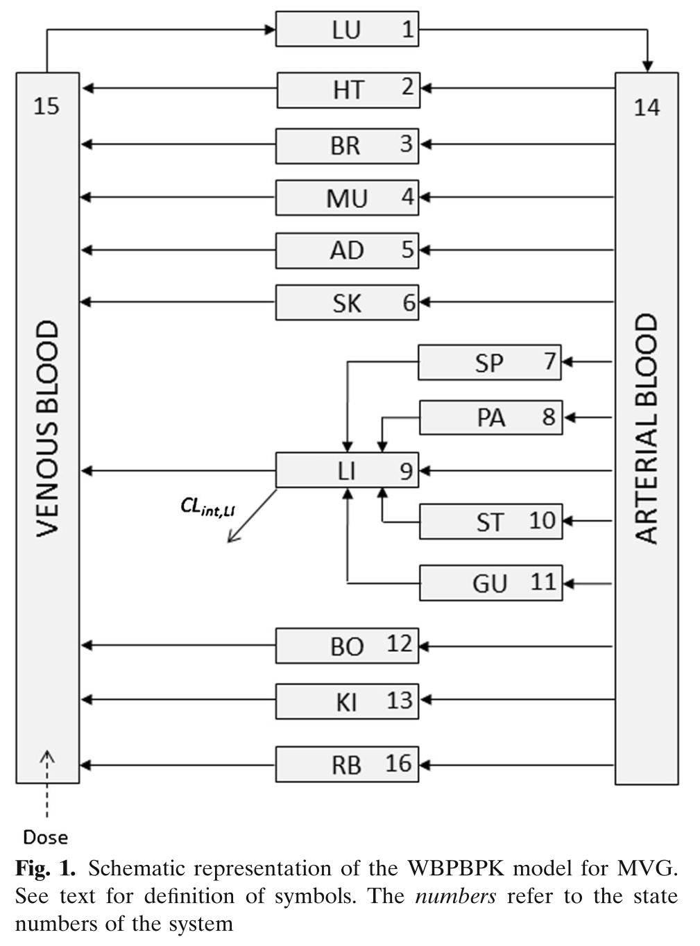
3.1.2.2 Physiologically-based PK
Building on the first simple example, we can be more ambitious, and try a full PBPK model. This one was published for mavoglurant (Wendling et al. 2016).
pbpk <- function(){
    ini({
        lKbBR  = 1.1
        lKbMU  = 0.3
        lKbAD  = 2
        lCLint = 7.6
        lKbBO  = 0.03
        lKbRB  = 0.3
        eta.LClint ~ 4
        add.err  <- 1
        prop.err <- 10
    })
    model({
        KbBR = exp(lKbBR)
        KbMU = exp(lKbMU)
        KbAD = exp(lKbAD)
        CLint= exp(lCLint + eta.LClint)
        KbBO = exp(lKbBO)
        KbRB = exp(lKbRB)

        ## Regional blood flows
        CO  = (187.00*WT^0.81)*60/1000;         # Cardiac output (L/h) from White et al (1968)
        QHT = 4.0 *CO/100;
        QBR = 12.0*CO/100;
        QMU = 17.0*CO/100;
        QAD = 5.0 *CO/100;
        QSK = 5.0 *CO/100;
        QSP = 3.0 *CO/100;
        QPA = 1.0 *CO/100;
        QLI = 25.5*CO/100;
        QST = 1.0 *CO/100;
        QGU = 14.0*CO/100;
        QHA = QLI - (QSP + QPA + QST + QGU); # Hepatic artery blood flow
        QBO = 5.0 *CO/100;
        QKI = 19.0*CO/100;
        QRB = CO - (QHT + QBR + QMU + QAD + QSK + QLI + QBO + QKI);
        QLU = QHT + QBR + QMU + QAD + QSK + QLI + QBO + QKI + QRB;

        ## Organs' volumes = organs' weights / organs' density
        VLU = (0.76 *WT/100)/1.051;
        VHT = (0.47 *WT/100)/1.030;
        VBR = (2.00 *WT/100)/1.036;
        VMU = (40.00*WT/100)/1.041;
        VAD = (21.42*WT/100)/0.916;
        VSK = (3.71 *WT/100)/1.116;
        VSP = (0.26 *WT/100)/1.054;
        VPA = (0.14 *WT/100)/1.045;
        VLI = (2.57 *WT/100)/1.040;
        VST = (0.21 *WT/100)/1.050;
        VGU = (1.44 *WT/100)/1.043;
        VBO = (14.29*WT/100)/1.990;
        VKI = (0.44 *WT/100)/1.050;
        VAB = (2.81 *WT/100)/1.040;
        VVB = (5.62 *WT/100)/1.040;
        VRB = (3.86 *WT/100)/1.040;

        ## Fixed parameters
        BP  = 0.61;      # Blood:plasma partition coefficient
        fup = 0.028;     # Fraction unbound in plasma
        fub = fup/BP;    # Fraction unbound in blood

        KbLU = exp(0.8334);
        KbHT = exp(1.1205);
        KbSK = exp(-.5238);
        KbSP = exp(0.3224);
        KbPA = exp(0.3224);
        KbLI = exp(1.7604);
        KbST = exp(0.3224);
        KbGU = exp(1.2026);
        KbKI = exp(1.3171);
        ##-----------------------------------------
        S15 = VVB*BP/1000;
        C15 = Venous_Blood/S15
        ##-----------------------------------------

        d/dt(Lungs)          = QLU*(Venous_Blood/VVB - Lungs/KbLU/VLU);
        d/dt(Heart)          = QHT*(Arterial_Blood/VAB - Heart/KbHT/VHT);
        d/dt(Brain)          = QBR*(Arterial_Blood/VAB - Brain/KbBR/VBR);
        d/dt(Muscles)        = QMU*(Arterial_Blood/VAB - Muscles/KbMU/VMU);
        d/dt(Adipose)        = QAD*(Arterial_Blood/VAB - Adipose/KbAD/VAD);
        d/dt(Skin)           = QSK*(Arterial_Blood/VAB - Skin/KbSK/VSK);
        d/dt(Spleen)         = QSP*(Arterial_Blood/VAB - Spleen/KbSP/VSP);
        d/dt(Pancreas)       = QPA*(Arterial_Blood/VAB - Pancreas/KbPA/VPA);
        d/dt(Liver)          = QHA*Arterial_Blood/VAB + QSP*Spleen/KbSP/VSP + QPA*Pancreas/KbPA/VPA + QST*Stomach/KbST/VST + QGU*Gut/KbGU/VGU - CLint*fub*Liver/KbLI/VLI - QLI*Liver/KbLI/VLI;
        d/dt(Stomach)        = QST*(Arterial_Blood/VAB - Stomach/KbST/VST);
        d/dt(Gut)            = QGU*(Arterial_Blood/VAB - Gut/KbGU/VGU);
        d/dt(Bones)          = QBO*(Arterial_Blood/VAB - Bones/KbBO/VBO);
        d/dt(Kidneys)        = QKI*(Arterial_Blood/VAB - Kidneys/KbKI/VKI);
        d/dt(Arterial_Blood) = QLU*(Lungs/KbLU/VLU - Arterial_Blood/VAB);
        d/dt(Venous_Blood)   = QHT*Heart/KbHT/VHT + QBR*Brain/KbBR/VBR + QMU*Muscles/KbMU/VMU + QAD*Adipose/KbAD/VAD + QSK*Skin/KbSK/VSK + QLI*Liver/KbLI/VLI + QBO*Bones/KbBO/VBO + QKI*Kidneys/KbKI/VKI + QRB*Rest_of_Body/KbRB/VRB - QLU*Venous_Blood/VVB;
        d/dt(Rest_of_Body)   = QRB*(Arterial_Blood/VAB - Rest_of_Body/KbRB/VRB);

        C15 ~ add(add.err) + prop(prop.err)
    })
}
This model estimates 6 structural parameters, 1 random effect, and includes combined additive and proportional residual error. The dependent variable, C15, is venous blood concentration.
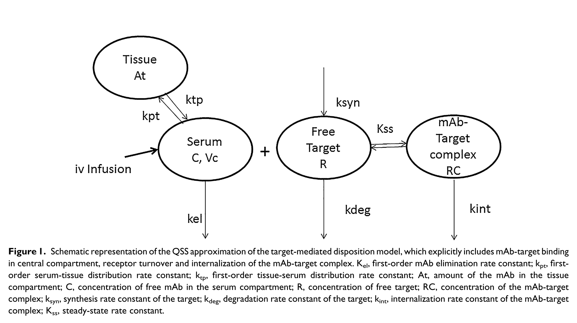
3.1.2.3 Nonlinear PK
Complex models can be estimated as well. In the example below, a target-mediated drug disposition PK model for nimotuzumab is illustrated (Rodríguez-Vera et al. 2015).
myPKPDModel <- function() {
ini({
tcl <- log(0.001)
tv1 <- log(1.45)
tQ <- log(0.004)
tv2 <- log(44)
tkss <- log(12)
tkint <- log(0.3)
tksyn <- log(1)
tkdeg <- log(7)
eta.cl ~ 2
eta.v1 ~ 2
eta.kss ~ 2
add.err <- 10
})
model({
cl <- exp(tcl + eta.cl)
v1 <- exp(tv1 + eta.v1)
Q <- exp(tQ)
v2 <- exp(tv2)
kss <- exp(tkss + eta.kss)
kint <- exp(tkint)
ksyn <- exp(tksyn)
kdeg <- exp(tkdeg)
k <- cl/v1
k12 <- Q/v1
k21 <- Q/v2
eff(0) <- ksyn/kdeg # initialize compartment
# Calculate concentration
conc = 0.5*(central/v1 - eff - kss) + 0.5*sqrt((central/v1 - eff - kss)**2 + 4*kss*central/v1)
d/dt(central) = -(k+k12)*conc*v1+k21*peripheral-kint*eff*conc*v1/(kss+conc)
d/dt(peripheral) = k12*conc*v1-k21*peripheral ##Free Drug second compartment amount
d/dt(eff) = ksyn - kdeg*eff - (kint-kdeg)*conc*eff/(kss+conc)
IPRED = log(conc)
IPRED ~ add(add.err)
})
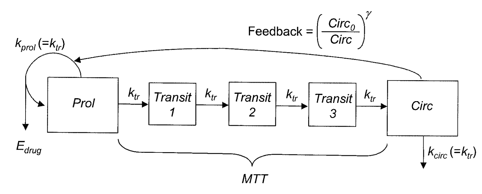
}3.1.2.4 PKPD models
Finally, we present an implementation of the Friberg myelosuppression model (Friberg et al. 2002). nlmixr is capable of handling almost any kind of model that can be implemented using ODEs.
wbc <- function() {
    ini({
        log_CIRC0 <- log(7.21)
        log_MTT   <- log(124)
        log_SLOPU <- log(28.9)
        log_GAMMA <- log(0.239)
        eta.CIRC0  ~ .1
        eta.MTT    ~ .03
        eta.SLOPU  ~ .2
        prop.err <- 10
    })
    model({
        CIRC0 = exp(log_CIRC0 + eta.CIRC0)
        MTT   = exp(log_MTT + eta.MTT)
        SLOPU = exp(log_SLOPU + eta.SLOPU)
        GAMMA = exp(log_GAMMA)

        # PK parameters from input dataset
        CL = CLI;
        V1 = V1I;
        V2 = V2I;
        Q = 204;

        CONC = A_centr/V1;

        # PD parameters
        NN    = 3;
        KTR   = (NN + 1)/MTT;
        EDRUG = 1 - SLOPU * CONC;
        FDBK  = (CIRC0 / A_circ)^GAMMA;

        CIRC = A_circ;

        A_prol(0) = CIRC0;
        A_tr1(0)  = CIRC0;
        A_tr2(0)  = CIRC0;
        A_tr3(0)  = CIRC0;
        A_circ(0) = CIRC0;

        d/dt(A_centr)  = A_periph * Q/V2 - A_centr * (CL/V1 + Q/V1);
        d/dt(A_periph) = A_centr * Q/V1 - A_periph * Q/V2;
        d/dt(A_prol)   = KTR * A_prol * EDRUG * FDBK - KTR * A_prol;
        d/dt(A_tr1)    = KTR * A_prol - KTR * A_tr1;
        d/dt(A_tr2)    = KTR * A_tr1 - KTR * A_tr2;
        d/dt(A_tr3)    = KTR * A_tr2 - KTR * A_tr3;
        d/dt(A_circ)   = KTR * A_tr3 - KTR * A_circ;

        CIRC ~ prop(prop.err)
    })
}
3.2 xpose.nlmixr
3.2.1 Introduction
xpose.nlmixr was written to provide an interface between nlmixr and the NONMEM-centric xpose model diagnostics package developed by Ben Guiastrennec and colleagues at Uppsala University.
3.2.2 Getting started
To get started, first install the package using:
devtools::install_github("nlmixrdevelopment/xpose.nlmixr")3.2.3 Overview
To leverage the full power of xpose to provide diagnostics for an nlmixr model, an xpose object must be created from the nlmixr fit.
xpdb <- xpose_data_nlmixr(nlmixrfit)This xpose object can now be used in the same way as any other - for full details, see the xpose website at uupharmacometrics.github.io/xpose.
3.3 shinyMixR
3.3.1 Introduction
The nlmixr package can be accessed through command line in R and RStudio, and through an interface shinyMixR supported by the nlmixr team. Both command line and interface support the integration with xpose.nlmixr.
shinyMixR aims to provide a user-friendly tool for nlmixr based on Shiny, which facilitates a workflow around an nlmixr project. The shinydashboard package was used to set up a structure for controlling and tracking runs with an nlmixr project, and was the basis for setting up the modular interface.
This project tool enhances the usability and attractiveness of nlmixr, facilitating dynamic and interactive use in real-time for rapid model development. In this project-oriented structure, the command line and dashboard can be used independently and/or interdependently. This means that many of the functions within the package can also be used outside the interface within an interactive R session.
Using shinyMixR, the user specifies and controls an nlmixr project workflow entirely in R. Within a project folder, a structure can be created to include separate folders for models, data and runs. Functionality is available to edit and execute a model code, summarize and compare model outputs in a tabular fashion, and view and compare model development using a tree paradigm. Inputs, outputs and metadata are stored in relation to the model code within the project structure (a discrete R object) to ensure traceability.
Results are visualized using modifications of existing packages (such as xpose.nlmixr, user-written functions and packages, or pre-existing plotting functionality included in the shinyMixR package. Results are reported using the R3port package in pdf and html format.
How the package can be used and what the most important functions are, is described in this part of the shinyMixR pkgdown site.
References
Wang, Yaning. 2007. “Derivation of various NONMEM estimation methods.” Journal of Pharmacokinetics and Pharmacodynamics 34 (5): 575–93. doi:10.1007/s10928-007-9060-6.
Wendling, Thierry, Nikolaos Tsamandouras, Swati Dumitras, Etienne Pigeolet, Kayode Ogungbenro, and Leon Aarons. 2016. “Reduction of a Whole-Body Physiologically Based Pharmacokinetic Model to Stabilise the Bayesian Analysis of Clinical Data.” The AAPS Journal 18 (1): 196–209. doi:10.1208/s12248-015-9840-7.
Rodríguez-Vera, Leyanis, Mayra Ramos-Suzarte, Eduardo Fernández-Sánchez, Jorge Luis Soriano, Concepción Peraire Guitart, Gilberto Castañeda Hernández, Carlos O. Jacobo-Cabral, Niurys De Castro Suárez, and Helena Colom Codina. 2015. “Semimechanistic model to characterize nonlinear pharmacokinetics of nimotuzumab in patients with advanced breast cancer.” Journal of Clinical Pharmacology 55 (8): 888–98. doi:10.1002/jcph.496.
Friberg, Lena E., Anja Henningsson, Hugo Maas, Laurent Nguyen, and Mats O Karlsson. 2002. “Model of chemotherapy-induced myelosuppression with parameter consistency across drugs.” Journal of Clinical Oncology 20 (24): 4713–21. doi:10.1200/JCO.2002.02.140.